Forward, backward, and hooks in PyTorch

A short notebook on what actually happens when you call .backward(), and how register_forward_hook and register_full_backward_hook let you peek into the chain rule.

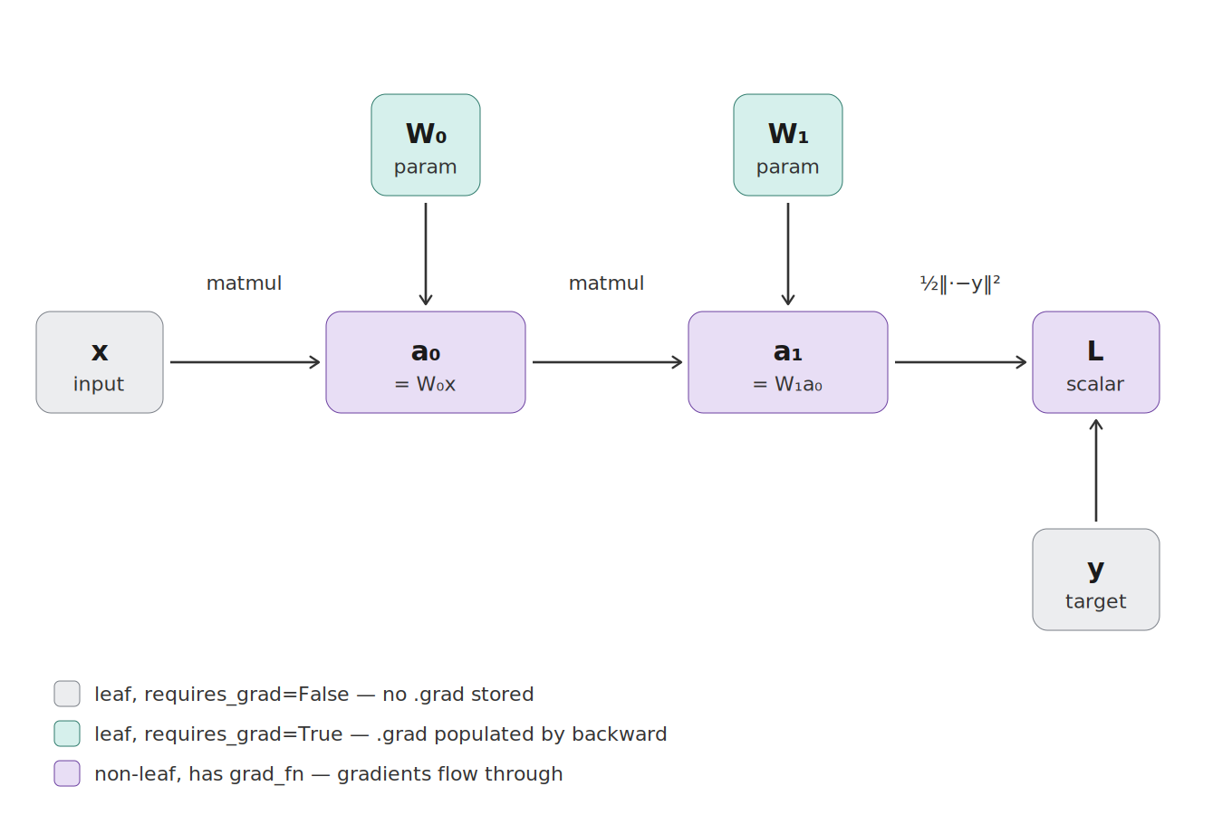
We’ll work with the smallest possible example — a two-layer linear network, no nonlinearity — so the graph has nothing hiding in it.

\[L \;=\; \tfrac{1}{2}\|a_1 - y\|^2, \qquad a_1 = W_1 a_0, \qquad a_0 = W_0 x\]

The forward pass

When you run model(x), PyTorch does two things at once:

1. Computes the actual numbers. Each operation (matmul, add, relu, …) takes tensors in, produces tensors out.

2. Builds a graph. Every tensor that is the output of an operation remembers which operation produced it and what the inputs were. This graph is the record that .backward() will later walk in reverse.

Tensors in that graph fall into three roles:

• Leaves with requires_grad=False (gray in the diagram): the input data x and target y. They entered the computation; nothing produced them.

• Leaves with requires_grad=True (teal): the model parameters W₀, W₁. Also not produced by any operation — they’re the things we want gradients for. After backward, their .grad attribute is populated.

• Non-leaves (purple): a₀, a₁, L. Each was produced by an operation and carries a grad_fn pointing back at the op and its inputs. Non-leaves don’t store .grad by default — gradients flow through them during backward but aren’t kept.

The backward pass

L.backward() walks the graph in reverse from L. At each node it asks: “for each of my inputs, what was the local derivative of me with respect to that input?” It multiplies that local derivative into the gradient flowing in from above (that’s the chain rule) and hands the result off to the input node, which repeats the process.

Define \(\delta_\ell := \partial L / \partial a_\ell\). Then:

\[\delta_1 = a_1 - y, \qquad \delta_0 = W_1^\top \delta_1, \qquad \partial L / \partial x = W_0^\top \delta_0\]

Each step is one Jacobian-vector product with the local Jacobian of that op.

At each linear layer, a second thing happens: the gradient also flows upward to the weight, producing a weight gradient of the form \(\delta \otimes (\text{input})\). These upward flows are what populate W.grad:

\[\frac{\partial L}{\partial W_1} = \delta_1 \otimes a_0, \qquad \frac{\partial L}{\partial W_0} = \delta_0 \otimes x\]

The reason it’s an outer product: in \(a = Wx\), each weight \(W_{ij}\) appears in exactly one output component \(a_i\), with coefficient \(x_j\). So \(\partial L / \partial W_{ij} = \delta_i \cdot x_j\), which is exactly the \((i, j)\) entry of the outer product \(\delta \otimes x\).

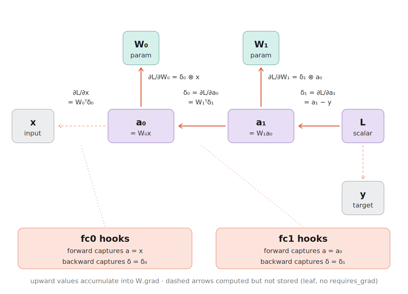
Things to notice in the backward diagram:

• The solid coral arrows land on teal boxes. Those are the stored gradients — W₀.grad and W₁.grad.

• The dashed coral arrows land on gray boxes. The gradient is computed (PyTorch has to evaluate \(W_0^\top \delta_0\) to propagate through the rest of the graph if there were any) but then thrown away because x is a leaf with requires_grad=False.

• Gradients through the purple intermediate nodes are transient. They flow through a₀, a₁ during backward but nothing stores them. If you wanted a₁.grad, you’d have to call a₁.retain_grad() before .backward().

The nn.Module hook API

PyTorch gives you three hooks on any nn.Module. Each one lets you run a callback at a specific point in the forward/backward lifecycle:

Hook	Registration	When it fires	Signature
Pre-forward	module.register_forward_pre_hook(fn)	Before module.forward() runs	fn(module, args) → optional modified args
Forward	module.register_forward_hook(fn)	After module.forward() returns	fn(module, args, output) → optional modified output
Backward	module.register_full_backward_hook(fn)	During .backward(), after gradients for this module are computed	fn(module, grad_input, grad_output) → optional modified grad_input

A few things to note:

• Pre-forward hooks are useful for inspecting or transforming inputs before they hit the module. For example, you could clamp activations or log input norms. If the hook returns a modified tuple, that becomes the new input to forward().

• Forward hooks see both the input and the output. Returning a value from the hook replaces the output — handy for feature extraction or on-the-fly patching.

• Backward hooks see grad_output (gradients flowing in from downstream) and grad_input (gradients flowing out to upstream). Returning a modified grad_input lets you alter gradient propagation.

• There is an older module.register_backward_hook() — it is deprecated and will be removed. Always use register_full_backward_hook instead; the “full” version handles multi-input/multi-output modules correctly.

• Every register_* call returns a RemovableHandle. Call handle.remove() when you’re done so the hook doesn’t fire on subsequent passes.

For capturing the \((a, \delta)\) factors we care about, we only need two of the three: a forward hook (to grab the input activation \(a\)) and a backward hook (to grab the error signal \(\delta\)). That’s what we use below.

Hooks on our two-layer network

Let’s see what the forward and backward hooks actually receive for layer fc₁ in our example.

Forward hook

For layer fc₁, when model(x) executes, the chain runs x → a₀ → a₁. At the moment fc₁’s forward finishes, the hook sees:

• input[0] = a₀ (the tensor that was fed into fc₁)

• output = a₁ (the tensor fc₁ just produced)

Save input[0]. That’s the \(a\) factor — the left-side label on fc₁’s hook box in the diagram.

Backward hook

Signature: fn_bwd(module, grad_input, grad_output).

It fires during backward, right after autograd computes gradients for this module. grad_output is a tuple of gradients flowing into the module’s outputs; grad_input is a tuple of gradients flowing out to the module’s inputs.

For fc₁, when backward reaches this layer, the relevant δ is the one at fc₁’s output — which is \(\delta_1 = \partial L / \partial a_1\). So the hook sees:

• grad_output[0] = \(\delta_1\) (what we want)

• grad_input[0] = \(W_1^\top \delta_1\) (the gradient that continues leftward)

Save grad_output[0]. That’s the \(\delta\) factor — the right-side label on fc₁’s hook box.

Putting the two together

With (a₀, δ₁) captured from fc₁, you can form the outer product yourself:

\[\delta_1 \otimes a_0 \;=\; \frac{\partial L}{\partial W_1}\]

which is exactly what ended up in W_1.grad — just recovered layer-by-layer instead of pre-summed. That’s the hook trick in one line.

Putting it together: hooks on a class-based MLP

A few details worth noting:

• The example uses a ReLU between the two linear layers, matching a more realistic MLP. The math we worked through still applies — ReLU just adds a mask step to the backward pass — and hooks on the linear layers still capture the right \((a, \delta)\) factors for each.

• x has shape (B, T, d_in) — a batch of B sequences, each of length T. nn.Linear treats any leading dimensions as batch dimensions, so the hooks capture tensors with (B, T, ...) shape. Both the batch and token dimensions are preserved — we haven’t aggregated anything away yet.

import torch
import torch.nn as nn
import torch.nn.functional as F


class MLP(nn.Module):
    def __init__(self, d_in, d_hidden, d_out):
        super().__init__()
        self.fc1 = nn.Linear(d_in, d_hidden, bias=False)
        self.fc2 = nn.Linear(d_hidden, d_out, bias=False)

    def forward(self, x):
        return self.fc2(F.relu(self.fc1(x)))


d_in, d_hidden, d_out = 4, 3, 2
B, T = 5, 6     # batch size, sequence length

torch.manual_seed(0)
x = torch.randn(B, T, d_in).requires_grad_(True)  # requires_grad silences a harmless hook warning
y = torch.randn(B, T, d_out)
model = MLP(d_in, d_hidden, d_out)

captured = {}
hooks = []


def make_fwd_hook(name):
    def fwd_hook(module, inp, out):
        captured[f"{name}_a"] = inp[0].detach().clone()
    return fwd_hook

hooks.append(model.fc1.register_forward_hook(make_fwd_hook("L1")))
hooks.append(model.fc2.register_forward_hook(make_fwd_hook("L2")))

def make_bwd_hook(name):
    def bwd_hook(module, grad_input, grad_output):
        captured[f"{name}_delta"] = grad_output[0].detach().clone()
    return bwd_hook

hooks.append(model.fc1.register_full_backward_hook(make_bwd_hook("L1")))
hooks.append(model.fc2.register_full_backward_hook(make_bwd_hook("L2")))


model.zero_grad()
loss = 0.5 * ((model(x) - y) ** 2).sum()
loss.backward()

for k, v in captured.items():
    print(f"  {k:10s}  shape {tuple(v.shape)}")

print(f"\nBatch (B={B}) and token (T={T}) dimensions are preserved in both hooks.")

# Clean up the hooks so they don't fire on subsequent forward/backward calls
for h in hooks:
    h.remove()

  L1_a        shape (5, 6, 4)
  L2_a        shape (5, 6, 3)
  L2_delta    shape (5, 6, 2)
  L1_delta    shape (5, 6, 3)

Batch (B=5) and token (T=6) dimensions are preserved in both hooks.

Reading the shapes:

• L1_a is (B, T, d_in) — the input activation to fc1, with batch and token dims intact.

• L1_delta is (B, T, d_hidden) — the gradient at fc1’s output.

• L2_a is (B, T, d_hidden) — the input to fc2, which is ReLU(fc1 output).

• L2_delta is (B, T, d_out) — the gradient at fc2’s output.

The outer product δ ⊗ a along the last two dims (with a sum over tokens) reconstructs the per-sequence weight gradient. Without summing over tokens, you have per-token factors — useful for packed-sequence work. Without summing over batch either, you have the full per-sample, per-token picture. The hooks capture everything; you choose what to aggregate and when.

Sanity check: does the reconstruction match W.grad?

Summing the outer product over both batch and token dimensions should recover the stored weight gradient exactly.

# Reconstruct fc2's weight gradient from the captured factors
# L2_delta: (B, T, d_out), L2_a: (B, T, d_hidden)
# Outer product per-token, then sum over B and T
g2_reconstructed = torch.einsum("bto,bti->oi", captured["L2_delta"], captured["L2_a"])
g1_reconstructed = torch.einsum("bth,bti->hi", captured["L1_delta"], captured["L1_a"])

print("fc1.weight.grad matches hook reconstruction:",
      torch.allclose(g1_reconstructed, model.fc1.weight.grad, atol=1e-6))
print("fc2.weight.grad matches hook reconstruction:",
      torch.allclose(g2_reconstructed, model.fc2.weight.grad, atol=1e-6))

fc1.weight.grad matches hook reconstruction: True
fc2.weight.grad matches hook reconstruction: True

Both match. The hook capture is the gradient in factored form — you just choose which dimensions to sum out when you want the stored .grad back.

Why Kronecker products show up

When PyTorch computes the weight gradient at a linear layer, it does this:

\[\text{grad}_W \;=\; \Delta^\top A\]

where \(A\) (shape B × d_in) and \(\Delta\) (shape B × d_out) are the stacked per-sample activations and errors — exactly what our hooks captured. That matmul is a sum of outer products \(\sum_t \delta_t a_t^\top\), but PyTorch never forms the individual outer products. It goes straight from the two factor tensors to the summed matrix in one GEMM.

The Kronecker product is just the vectorized version of the same structure. For a single sample, if you flatten the weight gradient matrix \(\delta a^\top\) column-by-column into a vector, you get:

\[\text{vec}(\delta \, a^\top) \;=\; a \otimes \delta\]

Concretely with \(\delta = [1, 2]\) and \(a = [3, 4, 5]\):

\[\begin{split}\delta \, a^\top = \begin{bmatrix} 3 & 4 & 5 \\ 6 & 8 & 10 \end{bmatrix} \quad\Rightarrow\quad \text{vec}(\ldots) = [3, 6, 4, 8, 5, 10] = a \otimes \delta\end{split}\]

The payoff is storage. For \(d_\text{in} = d_\text{out} = 4096\), the flattened gradient is \(1.7 \times 10^7\) numbers — but it’s fully determined by the two factors \((a, \delta)\), which are \(8192\) numbers total. The hooks expose exactly these factors, before PyTorch’s final matmul fuses them into W.grad.