Influence Functions: Where Does the Hessian Come From?#
A short derivation of the Koh & Liang (2017) influence function. We’ll then verify the formula numerically on a small MLP.
What we’d like to know#
A model is trained by minimising the empirical risk:
We want to know: how does each training point \(z\) affect the model’s loss on a particular test point \(z_{\text{test}}\)?
The cleanest way to formalise this is to imagine smoothly upweighting \(z\) by a small amount \(\varepsilon\):
When \(\varepsilon = 0\) we recover the original \(\hat\theta\). As \(\varepsilon\) grows, \(z\)’s loss matters more, and the optimum drifts.
The quantity we actually want is:
A positive value means upweighting \(z\) would increase the test loss (it’s hurting us); a negative value means it’s helping.
Step 1: chain rule#
The test loss \(L(z_{\text{test}}, \cdot)\) has no idea what \(\varepsilon\) is. It only depends on \(\varepsilon\) through the parameters that come out of training. So by the chain rule:
The first factor is a single backward pass through the model at the trained parameters. The second factor is the troublesome one: it asks how the learned parameters shift when we perturb the loss.
That’s hard because \(\hat\theta_{\varepsilon, z}\) is defined as an argmin. There’s no closed form. We can’t just differentiate it directly.
Step 2: differentiating through an argmin#
Even though we can’t write \(\hat\theta_{\varepsilon, z}\) in closed form, we know one thing about it: it’s a stationary point. The gradient of the perturbed objective vanishes there:
This is an implicit definition of \(\hat\theta_{\varepsilon, z}\). The trick — the implicit function theorem — is to differentiate this whole equation with respect to \(\varepsilon\), and then solve for \(d\hat\theta / d\varepsilon\).
Differentiating w.r.t. \(\varepsilon\) at \(\varepsilon = 0\) (where \(\hat\theta_{\varepsilon, z}\) becomes \(\hat\theta\)):
The Hessian shows up as the Jacobian of “take the gradient at \(\hat\theta_{\varepsilon, z}\)” with respect to \(\hat\theta_{\varepsilon, z}\) itself — that’s just the second derivative of the loss. It’s not chosen; it falls out of the chain rule applied to a vanishing-gradient condition.
Solving for the missing piece:
Step 3: assemble#
Plug back into the chain rule from Step 1:
This is the Koh & Liang influence function. Reading it left-to-right:
\(\nabla_\theta L(z, \hat\theta)\) — the “force” that upweighting \(z\) would exert on the loss landscape.
\(H_{\hat\theta}^{-1}\) — the compliance of the optimum: a Newton step that converts force into displacement. Sharp curvature ⇒ \(\hat\theta\) barely moves; flat curvature ⇒ it slides far.
\(\nabla_\theta L(z_{\text{test}}, \hat\theta)\) — the direction in parameter space the test loss is sensitive to.
The full expression dot-products them together: how much does the perturbation push \(\hat\theta\) in a direction the test loss cares about?
Connection to leave-one-out#
Removing point \(z\) from the training set is the same as setting its weight to \(0\) instead of \(1/n\) — i.e., upweighting by \(\varepsilon = -1/n\). So a first-order Taylor expansion gives:
This is what we’ll verify numerically below: predicted change vs. actual change after literally retraining without each point.
A small worked example#
Let’s verify the formula on a tiny MLP. We’ll:
Train a 2-layer MLP on a 2D synthetic classification problem.
Compute the influence of each training point on the loss at a single test point, using the formula above.
For comparison, retrain the model \(n\) times leaving each point out, and measure the actual test-loss change.
If the derivation is right, the predicted and actual changes should fall on the line \(y = x\).
We use L2 regularisation to keep the loss strongly convex enough that \(H_{\hat\theta}\) is well-conditioned and the local linearisation holds.
import torch
import torch.nn as nn
import numpy as np
import matplotlib.pyplot as plt

torch.manual_seed(0)
np.random.seed(0)

# Synthetic 2D binary classification: a noisy ring boundary
n = 60
X = torch.randn(n, 2)
y = ((X[:, 0] ** 2 + X[:, 1] ** 2) > 1.5).float().unsqueeze(1)

X_test = torch.randn(20, 2)
y_test = ((X_test[:, 0] ** 2 + X_test[:, 1] ** 2) > 1.5).float().unsqueeze(1)

print(f"Training set: {n} points, {int(y.sum())} positives")
Training set: 60 points, 26 positives
# A tiny MLP: 2 -> 8 -> 1
def make_model():
    torch.manual_seed(42)
    return nn.Sequential(
        nn.Linear(2, 8), nn.Tanh(),
        nn.Linear(8, 1),
    )

LAMBDA = 0.02     # L2 strength: keeps the loss strongly convex
bce = nn.BCEWithLogitsLoss(reduction="mean")

def total_loss(model, X_, y_, weights=None):
    # Mean BCE + L2.  `weights` lets us re-weight individual examples.
    logits = model(X_)
    if weights is None:
        loss = bce(logits, y_)
    else:
        per_ex = nn.functional.binary_cross_entropy_with_logits(
            logits, y_, reduction="none"
        ).squeeze()
        loss = (weights * per_ex).sum() / weights.sum()
    l2 = sum((p ** 2).sum() for p in model.parameters())
    return loss + LAMBDA * l2

def train(model, X_, y_, weights=None):
    # Train to (near) optimum with L-BFGS -- we want a true argmin.
    opt = torch.optim.LBFGS(
        model.parameters(), lr=0.1, max_iter=2000,
        tolerance_grad=1e-9, tolerance_change=1e-12,
        line_search_fn="strong_wolfe",
    )
    def closure():
        opt.zero_grad()
        loss = total_loss(model, X_, y_, weights)
        loss.backward()
        return loss
    opt.step(closure)
    return model

model = make_model()
train(model, X, y)
params = list(model.parameters())
n_params = sum(p.numel() for p in params)
print(f"Trained. {n_params} parameters total.")
Trained. 33 parameters total.
Computing \(H_{\hat\theta}^{-1}\)#
For a model this small we can afford the full Hessian. We get it row-by-row by differentiating each entry of the gradient vector.
(For real-world models with millions of parameters this is intractable; you’d use stochastic estimators like LiSSA or conjugate gradients — but the formula being computed is the same.)
def flat_grad(loss, params, create_graph=False):
    grads = torch.autograd.grad(loss, params, create_graph=create_graph)
    return torch.cat([g.reshape(-1) for g in grads])

# Hessian of the empirical loss at theta_hat
L_train = total_loss(model, X, y)
g_train = flat_grad(L_train, params, create_graph=True)

H = torch.zeros(n_params, n_params)
for i in range(n_params):
    H_row = torch.autograd.grad(g_train[i], params, retain_graph=True)
    H[i] = torch.cat([h.reshape(-1) for h in H_row])

H = 0.5 * (H + H.T)                                          # symmetrise
H_inv = torch.linalg.inv(H + 1e-4 * torch.eye(n_params))     # tiny damping
print(f"Hessian shape: {tuple(H.shape)}, cond(H) approx {torch.linalg.cond(H).item():.1f}")
Hessian shape: (33, 33), cond(H) approx 160.1
Influence of every training point on one test point#
# Pick a test point and get its gradient
test_idx = 0
x_te = X_test[test_idx:test_idx + 1]
y_te = y_test[test_idx:test_idx + 1]

g_test = flat_grad(bce(model(x_te), y_te), params).detach()

# Influence of each training point: I(z_i, z_test) = -g_test^T H^-1 g_i
predicted_influence = np.zeros(n)
for i in range(n):
    g_i = flat_grad(bce(model(X[i:i+1]), y[i:i+1]), params).detach()
    predicted_influence[i] = -(g_test @ H_inv @ g_i).item()

# Predicted change in test loss when removing point i: -I/n
predicted_change = -predicted_influence / n
Ground truth: actually retrain \(n\) times#
For each training point \(i\), we retrain from scratch with that point removed, then measure how much the test loss actually changed.
L_test_base = bce(model(x_te), y_te).item()

actual_change = np.zeros(n)
for i in range(n):
    mask = torch.ones(n)
    mask[i] = 0.0
    m_i = make_model()
    train(m_i, X, y, weights=mask)
    actual_change[i] = bce(m_i(x_te), y_te).item() - L_test_base

corr = np.corrcoef(predicted_change, actual_change)[0, 1]
print(f"Pearson correlation: {corr:.3f}")
Pearson correlation: 0.998
fig, ax = plt.subplots(figsize=(6, 6))
ax.scatter(predicted_change, actual_change, alpha=0.7)

lo = min(predicted_change.min(), actual_change.min())
hi = max(predicted_change.max(), actual_change.max())
ax.plot([lo, hi], [lo, hi], "k--", alpha=0.4, label="$y = x$")

ax.set_xlabel(r"Predicted change  ($-\mathcal{I}/n$)")
ax.set_ylabel("Actual change  (leave-one-out retrain)")
ax.set_title(f"Influence function vs. ground truth   (r = {corr:.3f})")
ax.legend()
ax.grid(alpha=0.3)
plt.tight_layout()
plt.show()
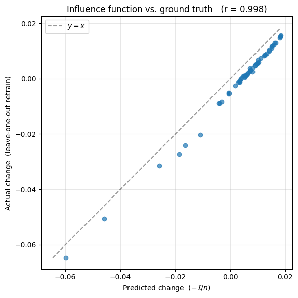
What this tells us#
The influence-function prediction tracks the actual leave-one-out change very closely — points sit near \(y = x\). Some points have positive influence (their removal increased the test loss; they were helping) and some have negative influence (they were hurting). The formula correctly identifies both, without ever retraining the model. The single Hessian inverse encodes everything we need to estimate the effect of removing any of the \(n\) training points.
A few things worth noting about why this works (and when it doesn’t):
Strong convexity matters. We added L2 regularisation to make the loss strongly convex around \(\hat\theta\). Without it, the Hessian can be singular or near-singular, and \(H^{-1}\) blows up. In practice people add a damping term \(H + \lambda I\) when applying this to non-convex models like deep neural networks.
The approximation is local. The derivation is a first-order Taylor expansion around \(\hat\theta\). If a single training point has a large effect — enough to move \(\hat\theta\) far — the linearisation breaks down. Outliers and high-influence points are exactly where the formula is least trustworthy.
Scaling up. For real networks the full Hessian has \(p^2\) entries with \(p\) in the millions. Two main strategies:
Hessian-vector products via LiSSA or conjugate gradients. You never form \(H\) explicitly, just compute \(H v\) for vectors \(v\), which costs one extra backward pass.
Approximations to \(H\). Gauss-Newton, empirical Fisher, or block-diagonal versions trade exactness for tractability.
The takeaway. The Hessian appears in the influence function for one reason: \(\hat\theta\) is an argmin, and the only way to differentiate through an argmin is via its first-order condition — and differentiating a gradient gives you a Hessian. Everything else is just chain rule.