Sparse autoencoders from scratch

Part 1 of a 4-part speedrun on sparse autoencoders (SAEs).

A sparse autoencoder (SAE) is an interpretability tool: it learns to re-express a language model’s internal activations as sparse combinations of features — directions in activation space that often correspond to human-recognisable concepts. That gives us a way to ask what a model is representing at any given token, to put names on the pieces, and even to intervene on them. Trained SAEs for many open models are hosted on Neuronpedia, where every latent gets its own dashboard — for example gemma-3-1b / layer-13 / gemmascope-2-res-16k / latent 7447, a “fruit” feature, shown with the texts it fires on, the tokens it promotes, and a human-readable label.

This notebook builds, from zero, everything needed to understand where a page like that comes from — why a model’s activations should decompose into nameable pieces at all, and how the thing that finds them is trained. By the end you will know:

• why features hide in the first place — networks store more features than they have dimensions (superposition), so single neurons respond to unrelated things and can’t be read directly;

• what an autoencoder is — and why the linear one can never do better than PCA, no matter how it’s trained;

• what makes superposition work — sparse features plus a nonlinearity, paying a price only when features co-fire;

• what an SAE actually is — an overcomplete dictionary trained to reconstruct activations through a sparsity penalty, whose decoder directions are the candidate features Neuronpedia puts names on;

• that it genuinely works — a trained SAE un-mixes activations built from a known dictionary and recovers the true feature directions;

• how SAEs are graded — L0, variance explained, and loss recovered, the numbers behind every dashboard.

Note: These are my own notes on the ARENA transformer interpretability material — these cover a small subset of the content and copy many of their fantastic exercises and explanations!

You can download this notebook and it should all run on CPU in about a minute.

What is a Sparse Autoencoder?

An autoencoder is one of the oldest ideas in representation learning: squeeze data through a narrow channel and force it to come out the other side intact. A sparse autoencoder — the tool this series is about — reuses that architecture almost verbatim, and then inverts the point of it.

Putting them side by side is the fastest way to see what changes. Here is where we are going — don’t worry about decoding every label yet; the whole notebook builds up to this picture, and we return to it at the end.

active sparse featuredense / mixed activationzero (inactive)reconstructed (approximate)

Left: the classical autoencoder squeezes its input through a narrower bottleneck, so it has no choice but to mix features together to survive the squeeze. Right: the sparse autoencoder runs the same machinery backwards: its input is already a dense mixture, its middle layer is wider than its input, and what limits it is not a shortage of dimensions but a sparsity constraint — all but a handful of latents must be zero. Highlighted edges show the subnetwork actually carrying signal.

The simplest autoencoder: an undercomplete linear autoencoder

The simplest autoencoder is linear — encoder and decoder are just matrices — and undercomplete — the latent dimension is smaller than the input, \(m < n\). Like every autoencoder, it is trained to reconstruct its own input. The encoder squeezes \(x \in \mathbb{R}^n\) down to \(h \in \mathbb{R}^m\); the decoder maps it back up:

\[ \underbrace{h = Ex}_{\text{encode}}, \qquad \underbrace{\hat{x} = Dh}_{\text{decode}}, \qquad E \in \mathbb{R}^{m \times n},\; D \in \mathbb{R}^{n \times m}. \]

The whole map is therefore \(\hat{x} = DEx = Ax\), with \(A = DE \in \mathbb{R}^{n\times n}\):

\[ \mathbb{R}^n \xrightarrow{\;E\;} \mathbb{R}^m \xrightarrow{\;D\;} \mathbb{R}^n . \]

All information passes through m = 2 numbers, so the composite A = DE has rank at most m — and every reconstruction is a mix of D's two columns, i.e. the model rebuilds everything from one shared 2-dimensional subspace.

Although \(A\) maps an \(n\)-dimensional input to an \(n\)-dimensional output, everything passes through the \(m\)-dimensional bottleneck, so \(\operatorname{rank}(A) \leq m\). The decoder’s side tells the same story: every reconstruction \(\hat{x} = Dh\) is a linear combination of the \(m\) columns of \(D\), so every possible output lies in the column space \(\operatorname{col}(D)\) — a single shared subspace of dimension at most \(m\), reused for every input.

Training means choosing \(E\) and \(D\) — equivalently, choosing a linear map \(A = DE\) of rank at most \(m\) — to minimise the average squared reconstruction error:

\[ \min_{\operatorname{rank}(A)\leq m}\; \mathbb{E}_{x}\big[\lVert x - Ax \rVert_2^2\big]. \]

In other words: the linear autoencoder looks for the best \(m\)-dimensional linear subspace in which to reconstruct the data.

Linear autoencoders recover the principal components

Skippable proof. The takeaway: training a linear bottleneck autoencoder is exactly PCA — it keeps the \(m\) directions of greatest variance and projects onto them, the best any rank-\(m\) map can do. Skim the pictures and the boxed result if you’d rather not derive it.

Which subspace wins? A projection’s error is whatever spread lies perpendicular to the subspace it keeps — so keep the directions where the data varies most. Those directions are the principal components, and rank reduction is exactly why they matter.

Concretely, here is the machine we’re claiming is optimal for \(m = 1\): the smallest autoencoder in this notebook, whose encoder row and decoder column are the same unit vector \(u_1\), the top principal direction —

— and here is what it does to a data cloud, stage by stage:

Encoding is a dot product: h = u₁ᵀx keeps only each point's coordinate along u₁ — one number. Decoding rebuilds x̂ = u₁h, so every reconstruction sits on the u₁ line, and the error x − x̂ (dashed) is exactly the component of x perpendicular to it. Keeping the line with the most variance along it leaves the least variance perpendicular to it — which is why the top principal component is precisely the right direction to keep when you cut rank.

Now the same statement in matrices. One housekeeping step first: our autoencoder has no bias terms, so every reconstruction \(\hat x = Ax\) must pass through the origin — we simply centre the data (subtract each feature’s mean) so the cloud sits there. Store the centred datapoints as the columns of \(X \in \mathbb{R}^{n \times N}\); training then solves

\[ \min_{\operatorname{rank}(A)\leq m} \lVert X - AX\rVert_F^2 \qquad (A = DE,\ \text{rank} \leq m\ \text{because of the bottleneck}), \]

with \(\lVert\cdot\rVert_F\) the elementwise \(L_2\) norm. Two standard facts, stated without proof:

1. Any matrix factors as \(X = U\Sigma V^\top\) — the SVD — with orthonormal columns in \(U\) and \(V\) and singular values \(\sigma_1 \geq \sigma_2 \geq \dots\) on \(\Sigma\)’s diagonal. For centred data, the columns of \(U\) are the principal components: the orthogonal directions of greatest variance, in decreasing order.

2. Eckart–Young: the closest rank-\(m\) matrix to \(X\) (in \(\lVert\cdot\rVert_F\)) is the truncated SVD, \(X_m = U_m\Sigma_mV_m^\top\) — keep the top \(m\) singular directions, drop the rest. (\(U_m\) = first \(m\) columns of \(U\).)

The proof, step by step

Claim: the optimal map is \(A^* = U_mU_m^\top\) — project every point onto the span of the top \(m\) principal directions.

Step 1: \(A^*\) produces the truncated SVD. Substitute \(X = U\Sigma V^\top\):

\[ A^*X = U_m\,\underbrace{U_m^\top U}_{?}\,\Sigma V^\top . \]

The matrix \(U_m^\top U\) is filled with dot products between singular vectors — and they are orthonormal, so each dot product is \(1\) on a match and \(0\) otherwise:

\[ U_m^\top U = [\,I_m \;\; 0\,] \qquad\text{(a selector: keep the first } m \text{ rows, kill the rest)} . \]

Applying that selector to \(\Sigma V^\top\) leaves exactly the top-\(m\) part:

\[ A^*X = U_m\,\Sigma_m V_m^\top = X_m . \]

Step 2: no admissible \(A\) does better. Any competitor satisfies \(\operatorname{rank}(A) \leq m\), and multiplying by \(X\) cannot raise rank, so its output \(AX\) is some matrix of rank \(\leq m\). But Eckart–Young says the closest such matrix to \(X\) is \(X_m\):

\[ \lVert X - AX\rVert_F \;\geq\; \lVert X - X_m\rVert_F \;=\; \lVert X - A^*X\rVert_F . \]

Every competitor is bounded below by the value \(A^*\) achieves — so \(A^*\) is optimal.

\[ \boxed{\,A^* = U_mU_m^\top,\qquad A^*X = X_m\,} \]

One optimal split is \(E = U_m^\top\), \(D = U_m\) (tied weights, \(D = E^\top\) — one matrix, both directions; we reuse this next section). The split isn’t unique — any invertible \(R\) gives \(E = RU_m^\top\), \(D = U_mR^{-1}\) with the same product — so reconstruction alone cannot pin down a basis inside the bottleneck. Hold that thought: an SAE faces the same freedom, and it is sparsity that breaks the tie.

Seeing it

The theorem says the network above — encoder \(u_1^\top\), decoder \(u_1\) — is what training should find. So check it both ways on a synthetic cloud: compute \(u_1\) from the SVD, and train a \(2 \to 1 \to 2\) linear autoencoder from random weights with plain gradient descent — then compare the direction the trained decoder learned against \(u_1\).

import numpy as np, matplotlib.pyplot as plt, torch
torch.manual_seed(0)
rng = np.random.default_rng(0)

# a centred 2-D cloud with lots of variance along one diagonal, little across it
X = rng.normal(size=(2, 200)) * np.array([[2.0], [0.45]])
th = np.deg2rad(30)
X = np.array([[np.cos(th), -np.sin(th)], [np.sin(th), np.cos(th)]]) @ X

# 1) the closed-form answer: u1 from the SVD
u1 = np.linalg.svd(X, full_matrices=False)[0][:, :1]
X_pca = u1 @ (u1.T @ X)                              # x̂ = u1 u1ᵀ x

# 2) the trained answer: a 2 -> 1 -> 2 linear autoencoder, plain MSE, random init
Xt = torch.tensor(X.T, dtype=torch.float32)
E = torch.nn.Linear(2, 1, bias=False)                # h  = E x
D = torch.nn.Linear(1, 2, bias=False)                # x̂ = D h
opt = torch.optim.Adam([*E.parameters(), *D.parameters()], lr=0.02)
for _ in range(800):
    loss = ((Xt - D(E(Xt))) ** 2).mean()
    opt.zero_grad(); loss.backward(); opt.step()

d = D.weight.detach().numpy(); d /= np.linalg.norm(d)   # the trained decoder's direction
fvu = lambda Xh: ((X - Xh) ** 2).sum() / (X ** 2).sum()
X_ae = D(E(Xt)).detach().numpy().T
print(f"cosine(trained direction, u1) = {abs((d.T @ u1).item()):.5f}")
print(f"variance lost — SVD: {fvu(X_pca):.2%},  trained autoencoder: {fvu(X_ae):.2%}")

fig, axes = plt.subplots(1, 2, figsize=(10.5, 4.6), sharex=True, sharey=True)

ax = axes[0]                                         # what goes IN
ax.scatter(*X, s=14, color="#4c8dd6", alpha=0.55)
ax.set_aspect("equal"); ax.grid(alpha=0.25, ls=":")
ax.set_title("input: the data $x$", fontsize=11)

ax = axes[1]                                         # what comes OUT
ax.scatter(*X, s=14, color="#4c8dd6", alpha=0.12, label="input (for reference)")
ax.scatter(*X_pca, s=16, color="#f08c00", alpha=0.9, label=r"reconstructions $\hat{x} = u_1 u_1^\top x$")
for i in range(0, 200, 12):                          # where a few points came from
    ax.plot([X[0, i], X_pca[0, i]], [X[1, i], X_pca[1, i]], color="0.65", lw=0.7, zorder=0)
ax.axline((0.0, 0.0), tuple(u1.ravel()), color="#f08c00", lw=1, alpha=0.6)
ax.axline((0.0, 0.0), tuple(d.ravel()), color="0.25", lw=1.4, ls="--", label="trained AE direction")
ax.set_aspect("equal"); ax.grid(alpha=0.25, ls=":")
ax.legend(loc="upper left", fontsize=9)
ax.set_title(r"output: every $\hat{x}$ collapses onto one line", fontsize=11)

fig.suptitle("SVD and gradient descent find the same line", y=1.0, fontsize=12)
plt.tight_layout(); plt.show()

cosine(trained direction, u1) = 1.00000
variance lost — SVD: 5.46%,  trained autoencoder: 11.84%

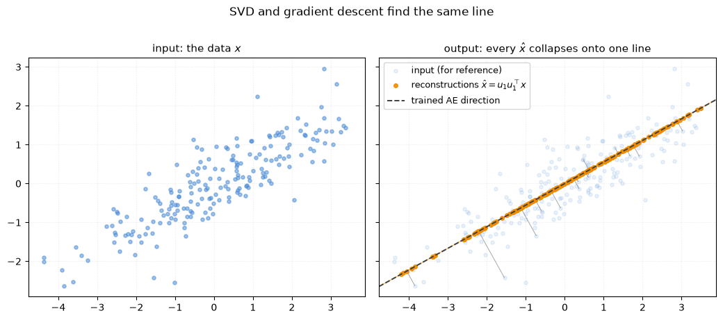
Gradient descent and the SVD find the same line, and no line does better:

\[ \boxed{ \text{undercomplete linear autoencoder} \quad\Longleftrightarrow\quad \text{projection onto the principal-component subspace} } \]

A linear autoencoder can therefore never represent more features than it has bottleneck dimensions. Beating that ceiling requires a nonlinearity — superposition, next.

How do ReLUs enable superposition?

Superposition means storing more features than you have dimensions, by letting the features share directions in activation space. We just proved a linear bottleneck cannot do this — \(\operatorname{rank}(A) \leq m\) — so something nonlinear has to give. Here is the smallest possible example.

The setup

A tiny tied-weight autoencoder: two input features squeezed through a one-dimensional bottleneck and back out again.

\[ x_A,\, x_B \;\longrightarrow\; h \;\longrightarrow\; \hat{x}_A,\, \hat{x}_B \]

\[ h = Wx, \qquad \hat{x} = W^\top h = W^\top W x \]

Two features, one number in the middle. The same weights are used to encode (+1, −1) and, transposed, to decode.

Sparsity

Consider that our data is sparse: features \(x_A\) and \(x_B\) are rarely on at the same time (they rarely “co-fire”). So in practice

\[\begin{split} x \approx \begin{bmatrix} 1 \\ 0 \end{bmatrix} \quad \text{or} \quad \begin{bmatrix} 0 \\ 1 \end{bmatrix} \end{split}\]

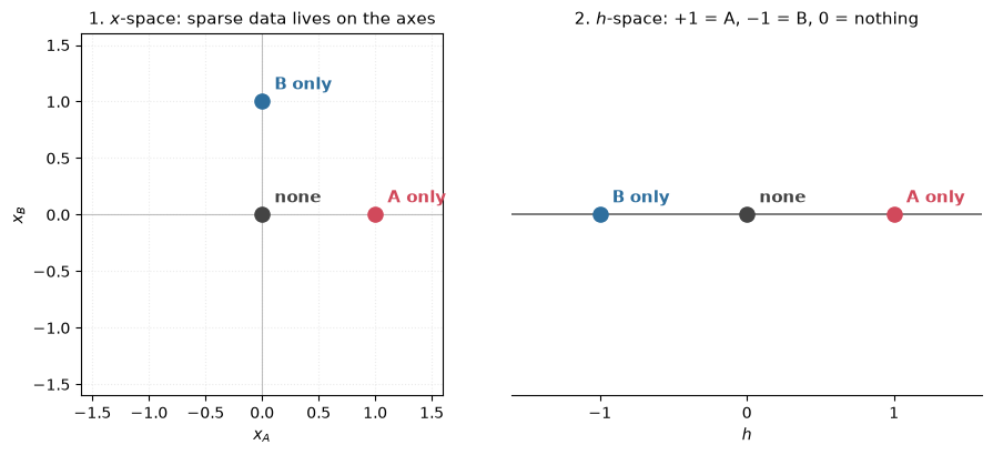
In \(x\)-space the data lives (almost) entirely on the two axes.

The bottleneck

Take \(W = \begin{bmatrix} 1 & -1 \end{bmatrix}\):

\[\begin{split} h = Wx = \begin{bmatrix} 1 & -1 \end{bmatrix} \begin{bmatrix} x_A \\ x_B \end{bmatrix} = x_A - x_B \end{split}\]

\[\begin{split} x = \begin{bmatrix} 1 \\ 0 \end{bmatrix} \Rightarrow h = 1, \qquad x = \begin{bmatrix} 0 \\ 1 \end{bmatrix} \Rightarrow h = -1 \end{split}\]

The sign of \(h\) tells us which feature is active. The two features land at \(+1\) and \(-1\), on opposite sides of the origin, and one scalar is carrying two features — that’s the superposition.

import numpy as np, matplotlib.pyplot as plt

W = np.array([[1.0, -1.0]])                       # the bottleneck: h = W x
labels = ["none", "A only", "B only"]              # sparse data: A and B never co-fire
X = np.array([[0.0, 0.0], [1.0, 0.0], [0.0, 1.0]])
colors = ["#444444", "#d1495b", "#2e6f9e"]
H = X @ W.T

fig, axes = plt.subplots(1, 2, figsize=(9.5, 4.2))

ax = axes[0]                                       # where the sparse data lives
ax.axhline(0, color="0.75", lw=0.8, zorder=0); ax.axvline(0, color="0.75", lw=0.8, zorder=0)
for lab, (px, py), c in zip(labels, X, colors):
    ax.scatter(px, py, s=90, color=c, zorder=3)
    ax.annotate(lab, (px, py), textcoords="offset points", xytext=(8, 8),
                color=c, fontsize=11, fontweight="bold")
ax.set_xlim(-1.6, 1.6); ax.set_ylim(-1.6, 1.6); ax.set_aspect("equal")
ax.set_xlabel("$x_A$"); ax.set_ylabel("$x_B$")
ax.set_title("1. $x$-space: sparse data lives on the axes", fontsize=11)
ax.grid(alpha=0.25, ls=":")

ax = axes[1]                                       # ...and where the bottleneck puts it
ax.axhline(0, color="0.4", lw=1.2, zorder=1)
for lab, v, c in zip(labels, H.ravel(), colors):
    ax.scatter(v, 0, s=90, color=c, zorder=3)
    ax.annotate(lab, (v, 0), textcoords="offset points", xytext=(8, 8),
                color=c, fontsize=11, fontweight="bold")
ax.set_xlim(-1.6, 1.6); ax.set_ylim(-1.0, 1.0)
ax.set_yticks([]); ax.set_xticks([-1, 0, 1]); ax.set_xlabel("$h$")
ax.set_title("2. $h$-space: $+1$ = A, $-1$ = B, $0$ = nothing", fontsize=11)
ax.spines[["left", "right", "top"]].set_visible(False)

fig.tight_layout(); plt.show()

The problem: interference

Because our weights are tied, \(\hat{x} = W^\top W x\):

\[\begin{split} \begin{bmatrix} \hat{x}_A \\ \hat{x}_B \end{bmatrix} = \begin{bmatrix} 1 & -1 \\ -1 & 1 \end{bmatrix} \begin{bmatrix} x_A \\ x_B \end{bmatrix} = \begin{bmatrix} x_A - x_B \\ x_B - x_A \end{bmatrix} \end{split}\]

But this causes problems:

\[\begin{split} x = \begin{bmatrix} 1 \\ 0 \end{bmatrix} \;\Rightarrow\; h = 1 \;\Rightarrow\; \hat{x} = \begin{bmatrix} 1 \\ -1 \end{bmatrix} \qquad \text{✗ wrong!} \end{split}\]

The \(-1\) is an interference term: the decoder cannot help but read the “\(A\) is on” signal as “\(B\) is negatively on”. (The culprit is the rank-1 bottleneck itself, not the weight tying — an untied linear decoder fails in exactly the same way.)

The fix

A ReLU (“rectified linear unit”) is the simplest nonlinearity there is: \(\operatorname{ReLU}(u) = \max(u, 0)\) — negative inputs become exactly zero, positive inputs pass through untouched.

If we add one after our decoder:

\[\begin{split} \mathrm{ReLU}\!\left(\begin{bmatrix} 1 \\ -1 \end{bmatrix}\right) = \begin{bmatrix} 1 \\ 0 \end{bmatrix} \qquad \text{✓ correct!} \end{split}\]

The interference lands on the negative side — not by luck, but by construction: we embedded the two features at \(+1\) and \(-1\), pointing in opposite directions, precisely so that each feature’s bleed-through into the other comes out negative. (Trained toy models discover the same antipodal arrangement on their own — we’ll watch it happen for real in the pentagon experiment below.) Features themselves are non-negative, so the nonlinearity clips the interference away:

\[ \hat{x} = \mathrm{ReLU}\left(W^\top W x\right) \]

One detail makes the answer come out exactly right: the columns of \(W\) have unit norm, so the surviving coordinate is already at the correct scale. ReLU deletes negative interference — it does not rescale what remains.

Where it still breaks

input	\(x\)	\(h = x_A - x_B\)	\(\hat{x} = W^\top W x\)	\(\hat{x} = \mathrm{ReLU}(W^\top W x)\)
none	\((0,0)\)	\(0\)	\((0,0)\) ✓	\((0,0)\) ✓
\(A\) only	\((1,0)\)	\(+1\)	\((1,-1)\) ✗	\((1,0)\) ✓
\(B\) only	\((0,1)\)	\(-1\)	\((-1,1)\) ✗	\((0,1)\) ✓
both	\((1,1)\)	\(0\)	\((0,0)\) ✗	\((0,0)\) ✗

ReLU is still wrong when features co-fire, but is correct otherwise. The input \((1,1)\) is indistinguishable from \((0,0)\) the moment it enters the bottleneck — \(h = 0\) for both — and no decoder can recover information that was destroyed upstream.

Takeaway

When your features are sparse (they rarely co-fire), you can use a bottleneck to compress them — but the compression creates interference. A ReLU removes the harmful negative interference; what remains are the collisions, which only occur when features fire together.

Get the causality straight: the sparsity here was a property of the data — we assumed features rarely co-fire. The ReLU does not create sparsity, and nothing about it makes activations sparse on its own; it is what lets the model exploit sparsity that is already there (and, inside an SAE later, what permits a latent to sit at exactly zero — the sparsity itself will come from an explicit penalty). This distinction recurs at every level of this notebook.

import numpy as np
import matplotlib.pyplot as plt

# h    = W x            with W = [1, -1]
# xhat = W^T h          (linear)  or  ReLU(W^T h)
W = np.array([[1.0, -1.0]])          # shape (1, 2)

labels = ["none", "A only", "B only", "both"]
X = np.array([
    [0.0, 0.0],   # none:   nothing on
    [1.0, 0.0],   # A only: just feature x_A
    [0.0, 1.0],   # B only: just feature x_B
    [1.0, 1.0],   # both:   features co-fire, violates sparsity
])
colors = ["#444444", "#d1495b", "#2e6f9e", "#7b9e2e"]

H         = X @ W.T                  # (4, 1)  bottleneck code
Xhat_lin  = H @ W                    # (4, 2)  xhat = W^T W x
Xhat_relu = np.maximum(Xhat_lin, 0)  # (4, 2)  xhat = ReLU(W^T W x)

for lab, x, h, xl, xr in zip(labels, X, H, Xhat_lin, Xhat_relu):
    print(f"{lab:7s}: x={x}  h={h[0]:+.0f}  xhat_lin={xl}  xhat_relu={xr}")


def scatter2d(ax, pts, title, xlabel, ylabel):
    ax.axhline(0, color="0.75", lw=0.8, zorder=0)
    ax.axvline(0, color="0.75", lw=0.8, zorder=0)
    seen = {}
    for lab, (px, py), c in zip(labels, pts, colors):
        ax.scatter(px, py, s=90, color=c, zorder=3)
        k = (round(px, 6), round(py, 6))          # stack labels when points coincide
        seen[k] = seen.get(k, 0) + 1
        ax.annotate(lab, (px, py), textcoords="offset points",
                    xytext=(8, 8 + 14 * (seen[k] - 1)), color=c,
                    fontsize=11, fontweight="bold")
    ax.set_xlim(-1.6, 1.6); ax.set_ylim(-1.6, 1.6)
    ax.set_aspect("equal")
    ax.set_xlabel(xlabel); ax.set_ylabel(ylabel)
    ax.set_title(title, fontsize=11)
    ax.grid(alpha=0.25, ls=":")


def scatter1d(ax, vals, title, xlabel):
    ax.axhline(0, color="0.4", lw=1.2, zorder=1)
    seen = {}
    for lab, v, c in zip(labels, vals.ravel(), colors):
        ax.scatter(v, 0, s=90, color=c, zorder=3)
        k = round(v, 6)
        seen[k] = seen.get(k, 0) + 1
        ax.annotate(lab, (v, 0), textcoords="offset points",
                    xytext=(8, 8 + 14 * (seen[k] - 1)), color=c,
                    fontsize=11, fontweight="bold")
    ax.set_xlim(-1.6, 1.6); ax.set_ylim(-1.0, 1.0)
    ax.set_yticks([]); ax.set_xticks([-1, 0, 1])
    ax.set_xlabel(xlabel)
    ax.set_title(title, fontsize=11)
    ax.spines[["left", "right", "top"]].set_visible(False)


fig, axes = plt.subplots(2, 2, figsize=(9.5, 8.5))

scatter2d(axes[0, 0], X, "1. $x$-space (input)", "$x_A$", "$x_B$")
scatter1d(axes[0, 1], H, "2. $h$-space (bottleneck), $h = x_A - x_B$", "$h$")
scatter2d(axes[1, 0], Xhat_lin,
          r"3. $\hat{x} = W^\top W x$  (no ReLU)", r"$\hat{x}_A$", r"$\hat{x}_B$")
scatter2d(axes[1, 1], Xhat_relu,
          r"4. $\hat{x} = \mathrm{ReLU}(W^\top W x)$", r"$\hat{x}_A$", r"$\hat{x}_B$")

fig.suptitle("How ReLUs enable superposition (2 features, 1 hidden unit, tied weights)",
             fontsize=13, y=0.98)
fig.tight_layout(rect=(0, 0, 1, 0.96))
plt.show()

none   : x=[0. 0.]  h=+0  xhat_lin=[0. 0.]  xhat_relu=[0. 0.]
A only : x=[1. 0.]  h=+1  xhat_lin=[ 1. -1.]  xhat_relu=[1. 0.]
B only : x=[0. 1.]  h=-1  xhat_lin=[-1.  1.]  xhat_relu=[0. 1.]
both   : x=[1. 1.]  h=+0  xhat_lin=[0. 0.]  xhat_relu=[0. 0.]

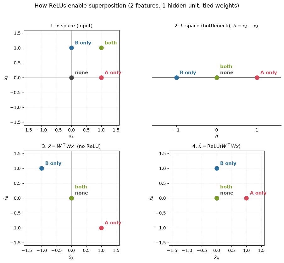
Reading the panels left-to-right, top-to-bottom: the four inputs start out distinct in \(x\)-space; the bottleneck collapses none and both onto the same value; the linear decoder pushes A only and B only off-axis into negative-interference territory; and the ReLU clips them back onto the correct axes, leaving only the none/both collision — the one error that was baked in before the decoder ever ran.

We hand-picked \(W\) for two features. Next, let a slightly bigger toy learn the same trick on its own — five features, two dimensions — and watch the geometry the linear representation hypothesis predicts actually emerge from training.

Scaling the toy up: five features, two dimensions

Suppose a model would “like” to represent \(n\) features but only has \(m < n\) dimensions to store them in. It cannot give every feature its own orthogonal axis. But if features are sparse (rarely active) and the model tolerates a little interference, it can do something clever: store the features as \(n\) non-orthogonal directions crammed into \(m\) dimensions. When only a few features are active at once, the interference between them is usually small enough to recover the signal.

The classic demonstration (Anthropic’s Toy Models of Superposition) is exactly the tied-weight toy we just built by hand — but with the weights learned, and forced to compress \(n\) sparse features through an \(m\)-dimensional bottleneck:

\[\mathbf{h} = W\mathbf{x}\ \ (\text{compress to } m),\qquad \hat{\mathbf{x}} = \operatorname{ReLU}(W^\top \mathbf{h} + \mathbf{b})\ \ (\text{decompress}).\]

\(W\) is \(m \times n\). The columns of \(W\) are the directions the model chooses for each feature. Let’s train it with \(n=5\) features squeezed into \(m=2\) dimensions and look at the geometry.

The toy model of §2. Five sparse features are squeezed through two hidden units and reconstructed. Because d < m, the features cannot be orthogonal — they share the two dimensions (superposition). Orange = an active feature; the encoder and decoder both reuse the same weight matrix W.

import numpy as np
import torch
import torch.nn as nn
import torch.nn.functional as F
import matplotlib.pyplot as plt

torch.manual_seed(0); np.random.seed(0)

class ToyModel(nn.Module):
    def __init__(self, n_features, n_hidden):
        super().__init__()
        self.W = nn.Parameter(torch.empty(n_hidden, n_features))
        nn.init.xavier_normal_(self.W)
        self.b = nn.Parameter(torch.zeros(n_features))
    def forward(self, x):
        h = x @ self.W.T                      # compress:  (batch, n_hidden)
        return F.relu(h @ self.W + self.b)    # decompress: (batch, n_features)

def generate_batch(batch, n_features, S):
    """Synthetic *sparse* feature vectors — the data the toy model must represent.

    Each of the `n_features` coordinates is, independently:
      - ON with probability `S`  (so on average only S·n_features fire at once), and
      - when ON, a random magnitude in (0, 1); when OFF, exactly 0.
    `S` is the key knob: the sparser the features, the more of them a d-dim
    bottleneck can pack into superposition without the interference swamping them.
    """
    is_on     = torch.rand(batch, n_features) < S   # e.g. [[False, False,  True, False, False]]
    magnitude = torch.rand(batch, n_features)        # e.g. [[0.549, 0.715, 0.603, 0.545, 0.424]]
    return magnitude * is_on                          # e.g. [[0.000, 0.000, 0.603, 0.000, 0.000]]

def train_toy(n_features, n_hidden, S, steps=6000, batch=1024, lr=1e-2):
    # Objective: plain reconstruction error (MSE). It's an autoencoder, so we simply ask
    # the output to match the input — no labels needed (exactly what an SAE does too).
    # Under the d < m bottleneck, minimising this is what forces superposition: the model
    # packs the sparse features into shared directions because, when they rarely collide,
    # that reconstructs them better on average than giving up and dropping them.
    model = ToyModel(n_features, n_hidden)
    opt = torch.optim.Adam(model.parameters(), lr=lr)
    for _ in range(steps):
        x = generate_batch(batch, n_features, S)
        loss = ((x - model(x)) ** 2).mean()
        opt.zero_grad(); loss.backward(); opt.step()
    return model

# 5 features, 2 hidden dims, high sparsity (each feature ON ~5% of the time)
model2d = train_toy(n_features=5, n_hidden=2, S=0.05)
W = model2d.W.detach()
print("feature vector norms:", W.norm(dim=0).numpy().round(2))

feature vector norms: [1.14 1.14 1.13 1.13 1.12]

fig, ax = plt.subplots(1, 2, figsize=(11, 4.4))

# (a) the 5 feature directions as 2D vectors
colors = plt.cm.viridis(np.linspace(0, 1, 5))
for i in range(5):
    ax[0].arrow(0, 0, W[0, i], W[1, i], head_width=0.04, color=colors[i], length_includes_head=True)
    ax[0].text(W[0, i]*1.15, W[1, i]*1.15, f"f{i}", color=colors[i], ha="center", va="center")
lim = 1.2
ax[0].set_xlim(-lim, lim); ax[0].set_ylim(-lim, lim); ax[0].set_aspect("equal")
ax[0].axhline(0, color="0.85", lw=.8); ax[0].axvline(0, color="0.85", lw=.8)
ax[0].set_title("5 features stored as directions in 2D")

# (b) the interference matrix WᵀW  (off-diagonal = feature overlap)
im = ax[1].imshow(W.T @ W, cmap="RdBu", vmin=-1, vmax=1)
ax[1].set_title(r"$W^\top W$: dot products between features")
ax[1].set_xticks(range(5)); ax[1].set_yticks(range(5))
plt.colorbar(im, ax=ax[1], fraction=0.046)
plt.tight_layout(); plt.show()

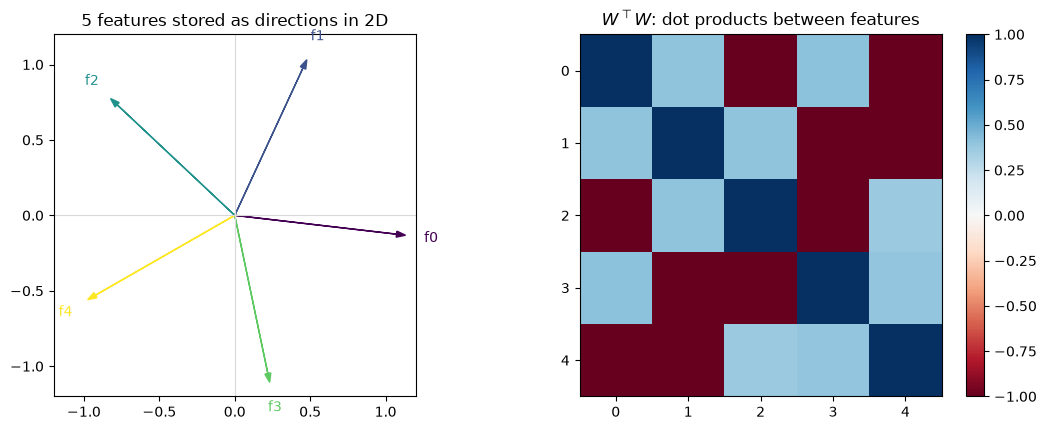
The model arranges the five features as spokes of a pentagon (or a similar symmetric arrangement). It cannot make them orthogonal — there are only two dimensions — so it spreads them out to minimise interference: the off-diagonal entries of \(W^\top W\) are small but non-zero. This is superposition in miniature. Two consequences that matter for the rest of the series:

• Each axis (neuron) is polysemantic. The x-axis has non-zero projection from several features at once. Reading neuron 0 tells you about a blend of features, not one.

• Sparsity is what makes it work. If many features were on simultaneously, the interference would swamp the signal. The sparser the features, the more you can pack in. (Try re-running with S=0.3 — the geometry collapses toward storing just two of the features orthogonally (which two is arbitrary), because interference is no longer affordable.)

Real language-model activations are the same story with \(d\) in the thousands and the number of features plausibly in the hundreds of thousands. We can’t read features off neurons. We need to learn the dictionary. Enter the SAE.

Everything so far ran in the compression direction: we knew the sparse features and watched them get squeezed into a dense \(h\) — by hand with two features, learned with five. A real network is the same story at scale — its activations are the dense \(h\) — except nobody hands us the sparse features that produced them. The next section runs the story backwards: given only \(h\), infer which features were active.

How is an SAE different? Running the map backwards

Note the reuse about to happen: the compressed code \(h\) of our autoencoders becomes the input of the sparse autoencoder. Interpretability hands us the middle of someone else’s autoencoder — the dense activations of a trained network — and asks what is stored in there. Let’s run the whole round trip with numbers small enough to check by hand.

The machine, up front

In case you skipped straight to this section: a sparse autoencoder is a one-hidden-layer autoencoder bolted onto a trained, frozen network. Pick a layer; at every token, tap the residual-stream activation \(h \in \mathbb{R}^m\) and feed it through an encoder and a decoder:

\[ z = \operatorname{ReLU}(W_{\text{enc}} h + b_{\text{enc}}), \qquad \hat h = W_{\text{dec}}\, z + b_{\text{dec}}, \]

with \(W_{\text{enc}} \in \mathbb{R}^{M \times m}\) and \(W_{\text{dec}} \in \mathbb{R}^{m \times M}\) — and, unusually for an autoencoder, \(M > m\): the hidden layer is wider than the input. Training minimises reconstruction error plus a sparsity penalty,

\[ \mathcal{L} = \lVert h - \hat h \rVert_2^2 + \lambda \lVert z \rVert_1. \]

The network being studied runs along the bottom and stays frozen — the SAE is a probe bolted on top at one chosen layer, changing nothing about the model. Bar height = number of dimensions: the encoder (weights, bias, ReLU) expands the tapped activation h into a latent vector z with far more dimensions, almost all of them zero; the decoder contracts it back to a reconstruction ĥ. Training pushes ĥ toward h while the λ‖z‖₁ term keeps z sparse.

Two choices should look strange after the last two sections: the middle layer is bigger than the input (what kind of bottleneck is that?), and sparsity is imposed by an extra loss term instead of being a property of the data we feed in. The rest of this section justifies both by running one concrete example end to end.

Step 1 — the network compresses (superposition)

A feature is a property of the input that a model has learned to represent — “this text is in French”, “the current token is a fruit”, “we’re inside a parenthetical”. The linear representation hypothesis says these features are encoded as directions in a model’s activation space: feature \(i\) has some unit vector \(\mathbf{d}_i \in \mathbb{R}^{d}\), and the activation vector for a given token is (approximately) a sparse weighted sum

\[\mathbf{x} \;\approx\; \mathbf{b} + \sum_i a_i\, \mathbf{d}_i,\qquad a_i \ge 0,\ \text{most } a_i = 0.\]

The scalar \(a_i\) is how strongly feature \(i\) is present. If this picture is right, then understanding a model means finding the dictionary \(\{\mathbf{d}_i\}\) and reading off which features fire where. That is exactly what an SAE tries to do.

The model’s natural basis — its individual neurons — is not the dictionary. A single neuron typically responds to many unrelated features (it is polysemantic), and a single feature is typically spread across many neurons. The reason is superposition.

Suppose the network reads text, and there are \(n = 4\) semantic features it wants to track:

	feature	fires on
1	cat	text about cats
2	dog	text about dogs
3	French	text written in French
4	CAPS	TEXT WRITTEN IN ALL CAPS

These are exactly the kind of features real language models track: each is sparse (most text is not about cats) and they co-occur freely (a French sentence about a cat is perfectly ordinary). But suppose the network has only \(m = 2\) residual-stream dimensions to store them in. Each feature gets a direction in that 2-D space; stack the four directions as the columns of

\[\begin{split} W_{\text{true}} = \begin{pmatrix} 1 & 0 & 0.7 & 0.7\\ 0 & 1 & 0.7 & -0.7 \end{pmatrix}, \qquad d_1 = \begin{pmatrix}1\\0\end{pmatrix},\; d_2 = \begin{pmatrix}0\\1\end{pmatrix},\; d_3 = \begin{pmatrix}0.7\\0.7\end{pmatrix},\; d_4 = \begin{pmatrix}0.7\\-0.7\end{pmatrix}, \end{split}\]

so \(d_1\) is the cat direction, \(d_2\) the dog direction, \(d_3\) the French direction, and \(d_4\) the CAPS direction. Four directions cannot all be orthogonal in two dimensions — they must overlap. That is superposition again, just \(4 \to 2\) instead of \(2 \to 1\).

This is the linear representation hypothesis from above, in miniature: each feature is a direction, and “how active it is” is how far the activation extends along it. The best evidence that the picture is right is that the directions can be used: steering — adding a multiple of \(d_3\) to the residual stream mid-forward-pass — makes the model behave as if the text were more French. Directions you can push on are directions the model actually listens to.

Four directions must share two dimensions, so they cannot all be orthogonal — that is the geometry of superposition. Per the linear representation hypothesis, the activation at any token is a weighted sum of whichever directions are active; pushing it further along d₃ (dashed) steers the model toward expressing that feature more.

From here on we write \(s\) for the vector of true feature activations — the \(x\) of the previous section — to emphasise that, from where we now stand, it is hidden. Now run the network over the sentence « le chat ». At the token chat, the cat and French features are on; dog and CAPS are off:

\[\begin{split} s = \begin{pmatrix}1\\0\\1\\0\end{pmatrix} \begin{matrix}\leftarrow \text{cat}\\ \leftarrow \text{dog}\\ \leftarrow \text{French}\\ \leftarrow \text{CAPS}\end{matrix} \end{split}\]

The residual-stream activation the network actually carries at that token is the sum of the active directions:

\[\begin{split} h = W_{\text{true}}\, s = d_{\text{cat}} + d_{\text{French}} = \begin{pmatrix}1\\0\end{pmatrix} + \begin{pmatrix}0.7\\0.7\end{pmatrix} = \begin{pmatrix}1.7\\0.7\end{pmatrix}. \end{split}\]

\[\begin{split} \underbrace{\begin{pmatrix}1\\0\\1\\0\end{pmatrix}}_{\text{sparse features } s} \;\longrightarrow\; \underbrace{\begin{pmatrix}1.7\\0.7\end{pmatrix}}_{\text{dense activation } h} \end{split}\]

Coordinates are not features

Look at \(h = (1.7,\, 0.7)\). Both coordinates are nonzero — but that does not mean two features are active, and the coordinates certainly don’t tell you which ones. There is no “cat coordinate” and no “French coordinate”: the first coordinate reads \(1.7\) because cat contributed \(1\) and French contributed \(0.7\), and a single feature like French (\(d_3 = (0.7,\, 0.7)\)) lights up both coordinates on its own.

The coordinates of \(h\) are just the model’s internal storage basis. The sparsity claim is not “the coordinates of \(h\) are usually zero” — they usually aren’t. The claim is:

there exists a different set of directions (\(d_{\text{cat}}, \dots, d_{\text{CAPS}}\)) whose activation coefficients (\(s\)) are sparse.

The SAE’s job is to find those directions.

Step 2 — the SAE decompresses (sparse inference)

The SAE is handed only \(h = (1.7,\, 0.7)\). It never sees \(s\) or \(W_{\text{true}}\) — it doesn’t even know the network is tracking cats. It computes the encoder–decoder pair from the top of the section:

\[ z = \operatorname{ReLU}(W_{\text{enc}} h + b_{\text{enc}}), \qquad \hat h = W_{\text{dec}}\, z + b_{\text{dec}}, \]

and it is trained so that \(\hat h \approx h\) while \(z\) stays sparse. If training succeeds, the columns of \(W_{\text{dec}}\) converge to the true feature directions — \(W_{\text{dec}} \approx W_{\text{true}}\) — and on our example

\[\begin{split} z \approx \begin{pmatrix}1\\0\\1\\0\end{pmatrix} = s, \qquad \hat h = W_{\text{dec}}\, z \approx d_{\text{cat}} + d_{\text{French}} = h. \end{split}\]

The SAE has un-mixed the activation: two numbers in, four numbers out, only two of them nonzero. Latent 1 has become a cat detector and latent 3 a French detector — each nonzero latent names one feature, which is exactly the kind of labelled, monosemantic latent you will browse on the Neuronpedia dashboard in Part 3.

Left: four feature directions d₁…d₄ share a two-dimensional residual stream, so they cannot all be orthogonal — that is superposition. On this input — the token chat in a French sentence — only d₁ (“cat”) and d₃ (“French”) are active (orange), and the network's activation is their sum h = (1.7, 0.7). Both coordinates of h are nonzero even though only two of the four features are on: coordinates are not features. Right: the same story as a pipeline. The network turns sparse s into dense h; the SAE, seeing only h, infers sparse latents z ≈ s and reconstructs ĥ ≈ h; latent 1 has become a “cat” detector, latent 3 a “French” detector. Its latent layer is wider than its input — the bottleneck is sparsity, not dimension.

Why the SAE latent space is bigger, not smaller

Notice the shape of the round trip. The network went \(4 \to 2\) (\(n\) features into \(m < n\) dimensions), so the SAE must go \(2 \to 4\): it needs more latents than input dimensions, \(M > m\) — one latent per feature it hopes to recover. A real SAE is the same picture scaled up: in Part 4 we expand Gemma’s \(m = 1152\) residual dimensions into \(M = 16384\) latents, each of which we hope is as nameable as “cat” or “French” — in Part 3 you will meet one that fires on fruit.

So an SAE is an overcomplete autoencoder. Its bottleneck is not “fewer numbers” — it has more numbers than its input. Its bottleneck is that most latents must be zero: an information bottleneck made of sparsity rather than dimensionality.

What actually creates the sparsity?

Nothing in \(z = \operatorname{ReLU}(W_{\text{enc}} h + b_{\text{enc}})\) forces \(z\) to be sparse. An overcomplete dictionary offers many ways to write \(\hat h \approx h\), and most of them smear the job across lots of small, dense activations. The ReLU only permits sparsity: it lets a latent sit at exactly zero and keeps the rest non-negative.

What rewards sparsity is an explicit term in the loss:

\[ \mathcal{L} = \underbrace{\lVert h - \hat h \rVert_2^2}_{\text{reconstruct } h} \;+\; \lambda\, \underbrace{\lVert z \rVert_1}_{\text{use few latents}}. \]

The two terms fight. Reconstruction says “use enough latents to rebuild \(h\)”; the \(L_1\) penalty makes every nonzero latent cost something, so reconstruction accuracy must pay for each latent it turns on. (Parts 1–2 replace the \(L_1\) term with better mechanisms — TopK, JumpReLU — but the tug-of-war is the same.)

Aside — a preview of JumpReLU

There is a subtler problem that a plain ReLU cannot fix, visible right here in our example. Take the most natural encoder — score each feature by dot product with its direction, \(a_i = d_i^\top h\) — and run it on \(h = d_1 + d_3\):

\[ a = W_{\text{true}}^\top h = (1.70,\;\; 0.70,\;\; 1.68,\;\; 0.70). \]

Every score is positive, so ReLU keeps all four: dog and CAPS appear to fire on a French sentence about a cat. Because the four directions overlap, active features leak into inactive detectors — and this time the leakage lands on the positive side, where clipping negatives does nothing. (Contrast the previous section, where the antipodal \(\pm 1\) embedding conveniently made all interference negative.)

What separates truth from leakage here is not sign but size: active scores \(\approx 1.7\), leakage \(= 0.7\). A ReLU with a per-latent threshold — exactly zero below \(\theta\), full value above it —

\[ \operatorname{JumpReLU}_\theta(a_i) = a_i \cdot \mathbb{1}[a_i > \theta] \]

with any \(\theta\) between \(0.7\) and \(1.68\) returns \((1.70,\; 0,\; 1.68,\; 0)\): the right two features, at full strength. That is JumpReLU, the activation GemmaScope uses. Part 2 shows why the threshold must be learned, and why keeping the full value (rather than subtracting \(\theta\)) matters.

The two networks, side by side again

This is the comparison the opening figure promised:

	Bottleneck autoencoder (toy model)	Sparse autoencoder
Input	sparse ground-truth features \(s\)	dense network activation \(h\)
Middle layer	narrower than input (\(m < n\))	wider than input (\(M > m\))
What limits it	dimension	sparsity penalty (most \(z_i = 0\))
Role of the ReLU	clips negative interference in the output	permits exact zeros in the latents
Shows	how superposition arises	how to undo it

\[ \boxed{\;\text{sparse features } s \;\overset{\text{superposition (the network)}}{\longrightarrow}\; \text{dense activation } h \;\overset{\text{sparse inference (the SAE)}}{\longrightarrow}\; \text{sparse latents } z \approx s\;} \]

That reversal is the entire reason SAEs exist.

One promise is still open: we claimed a trained SAE recovers the true directions. Time to prove it — with the field’s actual parametrization, on a dictionary we control.

Proving it: train an SAE against a known dictionary

The full anatomy (what GemmaScope actually parametrises)

Two renames and two new ingredients before we train for real. The walkthrough’s latents \(z\) are called \(\mathbf{f}\) from here on (the standard name), and the production parametrization adds a learned centre \(\mathbf{b}_{\text{dec}}\) and unit-norm dictionary rows.

An SAE is a second, wider autoencoder that we bolt onto a frozen model’s activations. It does not change the model; it just learns to re-express each activation vector \(\mathbf{x}\) as a sparse combination of dictionary directions. The architecture:

\[\begin{split} \begin{aligned} \text{encode:}\quad \mathbf{f} &= \sigma\!\big(W_{\text{enc}}(\mathbf{x}-\mathbf{b}_{\text{dec}}) + \mathbf{b}_{\text{enc}}\big) \\ \text{decode:}\quad \hat{\mathbf{x}} &= \mathbf{b}_{\text{dec}} + \sum_i f_i\, \mathbf{d}_i \quad(\mathbf{d}_i = \text{row } i \text{ of } W_{\text{dec}}) \end{aligned} \end{split}\]

• \(\mathbf{x} \in \mathbb{R}^{d_{\text{model}}}\) is one activation vector (e.g. a residual-stream vector at some layer and token).

• \(\mathbf{f} \in \mathbb{R}^{d_{\text{sae}}}\) are the latents (a.k.a. features), with \(d_{\text{sae}} \gg d_{\text{model}}\) — the dictionary is overcomplete. GemmaScope uses \(d_{\text{model}}=1152\) and \(d_{\text{sae}}=16384\) (a 14× expansion).

• The rows of \(W_{\text{dec}}\) are the dictionary directions \(\mathbf{d}_i\). They’re held to unit norm, so all the “how strongly is this feature present” information lives in \(\mathbf{f}\), not in the vector lengths.

• \(\sigma\) keeps latents non-negative — ReLU to start, JumpReLU in Part 2 — so they can sit at exactly zero. The sparsity itself comes from the loss below, not from \(\sigma\).

• \(\mathbf{b}_{\text{dec}}\) is subtracted before encoding and added back after — it acts as a learned “center” for the activations.

We train it on a single objective: reconstruct \(\mathbf{x}\) using as few active latents as possible.

The SAE of §3. The dictionary is overcomplete (d_sae ≫ d_model), so the encoder fans a 4-dim activation out to many latents — but only a handful are non-zero (orange). Reconstruction is the sum of just those few decoder directions (the bold orange edges), which is why x̂ = b + Σ fᵢ dᵢ stays sparse.

L0 vs L1: the central tension

The loss is the one we’ve been using all along — reconstruction plus \(\lambda\lVert\mathbf{f}\rVert_1\). The \(L_1\) term pushes activations toward zero, and because the \(L_1\) ball has corners, the minimum tends to land on solutions where most \(f_i\) are exactly zero.

Why \(L_1\) and not “count the non-zeros”? Because the thing we actually care about is the \(L_0\) “norm” — the number of active latents:

\[\lVert \mathbf{f}\rVert_0 \;=\; \#\{i : f_i \neq 0\}.\]

\(L_0\) is exactly “how many features fired”, which is what interpretability cares about — but it’s piecewise-constant, so its gradient is zero almost everywhere and useless for training. \(L_1\) is the convex surrogate whose gradient is non-zero almost everywhere and does induce sparsity. This gap between “the \(L_0\) we want” and “the \(L_1\) we can optimise” is the single most important tension in SAE design, and it’s what motivates JumpReLU in Part 2. Remember the phrase “L0” — on the Neuronpedia dashboard it’s the average number of latents active per token, and it’s the headline number for how interpretable an SAE is.

Watching an SAE recover features from superposition

To prove the SAE does what we claim, we need ground truth, so we generate activations from a known dictionary (these activations play the role of the toy model’s bottleneck \(\mathbf{h}\) from the pentagon experiment — the compressed vector an SAE actually sees).

Setup: \(n_{\text{true}}=32\) ground-truth feature directions in a \(d=16\)-dim space (genuinely in superposition, \(32 > 16\)). Each data point turns on ~3 random features with known positive magnitudes and sums their directions — precisely the generative model the SAE assumes, so a good SAE should rediscover the 32.

torch.manual_seed(0)
d, n_true, d_sae = 16, 32, 64
D_true = F.normalize(torch.randn(n_true, d), dim=-1)   # ground-truth dictionary (unit rows)
p_active = 3.0 / n_true                                 # ~3 active features per example

def gen(batch):
    mask = (torch.rand(batch, n_true) < p_active).float()
    mags = (0.5 + torch.rand(batch, n_true)) * mask     # magnitude ~ U(0.5, 1.5) when ON
    return mags @ D_true, mags                          # x = sum of active feature directions

class ReLUSAE(nn.Module):
    def __init__(self, d_model, d_sae):
        super().__init__()
        self.b_dec = nn.Parameter(torch.zeros(d_model))
        self.W_enc = nn.Parameter(torch.randn(d_model, d_sae) / np.sqrt(d_model))
        self.b_enc = nn.Parameter(torch.zeros(d_sae))
        self.W_dec = nn.Parameter(F.normalize(torch.randn(d_sae, d_model), dim=-1))
    @torch.no_grad()
    def normalize_decoder(self):
        self.W_dec.data = F.normalize(self.W_dec.data, dim=-1)
    def forward(self, x):
        f = F.relu((x - self.b_dec) @ self.W_enc + self.b_enc)   # encode (ReLU)
        return f @ self.W_dec + self.b_dec, f                    # decode

def train_relu_sae(sae, l1=0.4, steps=2000, batch=4096, lr=4e-3):
    opt = torch.optim.Adam(sae.parameters(), lr=lr)
    for _ in range(steps):
        x, _ = gen(batch)
        x_hat, f = sae(x)
        loss = ((x_hat - x) ** 2).sum(-1).mean() + l1 * f.abs().sum(-1).mean()
        opt.zero_grad(); loss.backward(); opt.step()
        sae.normalize_decoder()          # keep dictionary directions unit-norm
    return sae

sae = train_relu_sae(ReLUSAE(d, d_sae))

# how many active latents per example (L0), and reconstruction quality (FVU)?
x, mags = gen(8192)
x_hat, f = sae(x)
L0  = (f > 1e-6).float().sum(-1).mean().item()
FVU = (((x_hat - x) ** 2).sum() / ((x - x.mean(0)) ** 2).sum()).item()
print(f"L0 (avg active latents) = {L0:.2f}   (true value ~ {p_active*n_true:.1f})")
print(f"FVU (fraction of variance unexplained) = {FVU:.3f}   ->  {1-FVU:.1%} of variance explained")

L0 (avg active latents) = 8.71   (true value ~ 3.0)
FVU (fraction of variance unexplained) = 0.125   ->  87.5% of variance explained

# Did we recover the true dictionary? Match each true feature to its best SAE latent by cosine.
cos = F.normalize(D_true, dim=-1) @ F.normalize(sae.W_dec.detach(), dim=-1).T   # (n_true, d_sae)
best_cos = cos.max(dim=1).values
recovered = (best_cos > 0.9).float().mean().item()
print(f"{recovered:.0%} of the {n_true} true features recovered with cosine > 0.9")

plt.figure(figsize=(7, 3.2))
plt.hist(best_cos.numpy(), bins=24, range=(0, 1), color="darkorange", edgecolor="white")
plt.axvline(0.9, color="k", ls="--", lw=1); plt.xlabel("cosine(true feature, best SAE latent)")
plt.ylabel("# true features"); plt.title("SAE recovers the ground-truth dictionary")
plt.tight_layout(); plt.show()

72% of the 32 true features recovered with cosine > 0.9

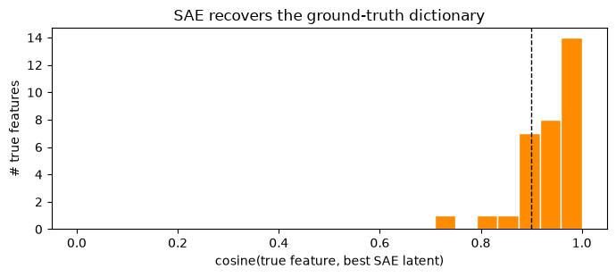
About three-quarters of the true directions come back with cosine > 0.9 — the SAE has largely un-mixed the superposition, turning polysemantic 16-dimensional vectors into a mostly-monosemantic 64-latent code. That’s the whole game — though not played perfectly: it spends ~9 latents per example where the true answer is ~3.

Two things to notice, because they’re the seeds of Part 2:

• L0 is measured, not set. We chose \(\lambda\) (the \(L_1\) coefficient) and observed an L0 of ~9 — three times the true count. To hit a target L0 you have to hunt for the right \(\lambda\). JumpReLU will let us target L0 directly.

• Not every true feature is recovered perfectly, and some SAE latents are duplicates or dead. Both are real failure modes we’ll meet again.

The metrics that grade an SAE

Three numbers summarise any SAE, and you’ll see all three throughout the series:

Metric	Definition	What it tells you
L0	avg. number of latents active per token, \(\mathbb{E}\lVert\mathbf{f}\rVert_0\)	sparsity / interpretability. Lower = each token explained by fewer features. GemmaScope’s layer-13 SAE targets L0 ≈ 60.
Reconstruction (FVU / variance explained)	\(\mathbb{E}\lVert\mathbf{x}-\hat{\mathbf{x}}\rVert_2^2 / \mathbb{E}\lVert\mathbf{x}-\bar{\mathbf{x}}\rVert_2^2\)	fidelity. How much of the activation the SAE captures.
Loss recovered (CE / delta)	how much of the model’s next-token loss survives when you replace \(\mathbf{x}\) with \(\hat{\mathbf{x}}\)	fidelity that matters to the model — a reconstruction can look good in MSE but still hurt the model’s predictions. We’ll compute this on real Gemma in Part 4.

L0 and reconstruction are in fundamental tension: driving L0 down (fewer active latents) always costs reconstruction. Every SAE lives somewhere on this Pareto frontier, and the whole point of better architectures (Part 2) is to push the frontier outward — same reconstruction at lower L0.

Two more diagnostics worth knowing:

• Dead latents — latents that (almost) never fire on any input. Wasted dictionary capacity; training tricks like resampling revive them.

• Feature density — for each latent, the fraction of tokens it fires on. This is literally the “activation density” number on the dashboard, and we’ll compute it for the fruit feature in Part 3.

Where we are

Everything the rest of the series leans on, in six lines:

1. a linear bottleneck autoencoder can only project onto its top-\(m\) principal subspace — it cannot store more features than dimensions;

2. a ReLU lets a bottleneck exploit sparsity to store more features than dimensions, paying only when features co-fire — that is superposition, and it is why neurons are polysemantic and features are directions we must learn;

3. a sparse autoencoder runs the process in reverse: an overcomplete dictionary trained with reconstruction + a sparsity penalty, whose decoder rows are the learned feature directions;

4. it works, imperfectly: on a known dictionary, a plain ReLU SAE recovers ~72% of the true directions at cosine > 0.9, while overspending latents (L0 ≈ 9 vs a true ~3) — exactly the slack better architectures close;

5. the sparsity we care about is L0 (a count); the penalty we can train is L1 — that mismatch, plus the way \(L_1\) drags down the very latents that should fire (shrinkage), is the theme of Part 2;

6. an SAE is graded on L0, reconstruction (FVU), and loss recovered, and lives on an L0-versus-fidelity frontier that better architectures push outward.

Next → Part 2: SAE architectures & JumpReLU — TopK, Gated, and the JumpReLU activation GemmaScope actually uses, with its straight-through-estimator gradients implemented by hand.