

Training your own JumpReLU SAE on Gemma 3 1B#
Part 4 of 4 — the payoff. We’ve dissected superposition (Part 1), built and understood JumpReLU
(Part 2), and reverse-engineered a real dashboard (Part 3). Now we train our own GemmaScope-style
JumpReLU SAE from scratch on gemma-3-1b-pt, at the same layer-13 residual stream, from a
subset of The Pile — and check it actually discovers interpretable features.
We deliberately do not reach for sae_lens or transformer_lens: the whole point is to see
every moving part. The pipeline is exactly four stages:
Collect activations — hook the residual stream, stream text, build a big activation buffer.
Define the SAE — the trainable JumpReLU from Part 2, scaled up to
d_sae = 16384.Train — reconstruction + L0 penalty, with the tricks that make it actually work (chiefly a separate high LR for the threshold, plus activation normalisation).
Evaluate & interpret — L0, variance-explained, loss-recovered, and the monosemantic features it found — compared head-to-head with the official GemmaScope-2 SAE.
GPU + gated-model access required (won’t run in the site build)
These cells load google/gemma-3-1b-pt, collect ~3M activations and train a 16k-latent SAE — a
few minutes on a big GPU (this run was an NVIDIA B300). They’re marked not to execute during
the site build; the outputs shown were produced live. To reproduce: accept the Gemma license,
huggingface-cli login, pip install transformers datasets safetensors, run top to bottom.
Stage 1 — Collect residual-stream activations#
An SAE’s training data is not text — it’s the activation vectors the model produces. We hook
the output of block 13 (model.layers.13.output, the canonical mid-layer residual stream), stream
text from The Pile, and fill a buffer of a few million d_model = 1152-dim vectors. Two details
that matter a lot in practice:
Drop the BOS token. Its residual is a massive-norm outlier (“attention sink”) that would dominate the loss and distort the learned dictionary.
Normalise the scale. Gemma’s residuals have norm ~10⁴; we rescale so \(\mathbb{E}\lVert x\rVert = \sqrt{d_{\text{model}}}\). This puts activations in a sane range so a single sparsity coefficient and threshold work across latents (GemmaScope does the same).
import torch, torch.nn as nn, torch.nn.functional as F, numpy as np, time, collections
import matplotlib.pyplot as plt
from transformers import AutoModelForCausalLM, AutoTokenizer
from datasets import load_dataset
from huggingface_hub import hf_hub_download
from safetensors.torch import load_file

DEV = "cuda"
MODEL_ID, LAYER, D_MODEL, D_SAE = "google/gemma-3-1b-pt", 13, 1152, 16384
torch.manual_seed(0)

tok = AutoTokenizer.from_pretrained(MODEL_ID)
model = AutoModelForCausalLM.from_pretrained(MODEL_ID, dtype=torch.bfloat16, device_map=DEV).eval()

class ResidCatcher:
    def __init__(self, model, layer):
        self.acts = None
        self.h = model.model.layers[layer].register_forward_hook(self._hook)
    def _hook(self, m, i, o): self.acts = (o[0] if isinstance(o, tuple) else o).detach()
    def remove(self): self.h.remove()
cat = ResidCatcher(model, LAYER)

@torch.no_grad()
def resid_of(ids, am=None):
    model(input_ids=ids, attention_mask=am); return cat.acts.float()

SEQ, BATCH, N_TOKENS = 128, 128, int(3e6)
ds = load_dataset("monology/pile-uncopyrighted", split="train", streaming=True); it = iter(ds)
def next_texts(n):
    out = []
    while len(out) < n:
        ex = next(it)
        if len(ex["text"]) > 200: out.append(ex["text"])
    return out

t0 = time.time()
buf = torch.empty(N_TOKENS, D_MODEL, dtype=torch.bfloat16, device=DEV); n = 0
while n < N_TOKENS:
    enc = tok(next_texts(BATCH), return_tensors="pt", truncation=True, max_length=SEQ, padding="max_length")
    ids = enc.input_ids.to(DEV); am = enc.attention_mask.to(DEV)
    x = resid_of(ids, am)
    keep = am.bool() & (ids != tok.bos_token_id)              # drop pads AND the BOS outlier
    v = x[keep]; take = min(v.shape[0], N_TOKENS - n)
    buf[n:n+take] = v[:take].bfloat16(); n += take
scale = (D_MODEL ** 0.5) / buf.float().norm(dim=-1).mean().item()
print(f"collected {n} activations in {time.time()-t0:.0f}s | mean‖x‖→√d via scale={scale:.5f}")
collected 3000000 activations in 27s | mean‖x‖→√d via scale=0.00332
Stage 2 — The trainable JumpReLU SAE#
This is the Part-2 architecture at scale: encoder → JumpReLU (with straight-through gradients on
the learned per-latent threshold) → decoder, with unit-norm decoder rows. At inference it will
be identical to the GemmaScope SAE we loaded in Part 3; the STE only exists to train log_theta.
def rectangle(x): return (x.abs() < 0.5).float()

class JumpReLUf(torch.autograd.Function):        # forward z·1[z>θ]; STE grad on θ
    @staticmethod
    def forward(ctx, z, th, eps): ctx.save_for_backward(z, th); ctx.eps = eps; return z * (z > th).float()
    @staticmethod
    def backward(ctx, g):
        z, th = ctx.saved_tensors; e = ctx.eps
        return (z > th).float() * g, -(th / e) * rectangle((z - th) / e) * g, None

class Heavisidef(torch.autograd.Function):       # forward 1[z>θ] (the L0 count); STE grad on θ
    @staticmethod
    def forward(ctx, z, th, eps): ctx.save_for_backward(z, th); ctx.eps = eps; return (z > th).float()
    @staticmethod
    def backward(ctx, g):
        z, th = ctx.saved_tensors; e = ctx.eps
        return 0.0 * g, -(1.0 / e) * rectangle((z - th) / e) * g, None

class JumpReLUSAE(nn.Module):
    def __init__(self, d_model, d_sae, eps=0.1, theta0=0.1):
        super().__init__(); self.eps = eps
        self.b_dec = nn.Parameter(torch.zeros(d_model))
        self.W_dec = nn.Parameter(F.normalize(torch.randn(d_sae, d_model), dim=-1))
        self.W_enc = nn.Parameter(self.W_dec.data.T.clone())          # tied init
        self.b_enc = nn.Parameter(torch.zeros(d_sae))
        self.log_theta = nn.Parameter(torch.full((d_sae,), float(np.log(theta0))))
    @property
    def theta(self): return self.log_theta.exp()
    @torch.no_grad()
    def normalize_decoder(self): self.W_dec.data = F.normalize(self.W_dec.data, dim=-1)
    def encode(self, x):
        z = F.relu((x - self.b_dec) @ self.W_enc + self.b_enc)
        return JumpReLUf.apply(z, self.theta, self.eps), z
    def forward(self, x):
        acts, z = self.encode(x); return acts @ self.W_dec + self.b_dec, acts, z

sae = JumpReLUSAE(D_MODEL, D_SAE).to(DEV)
print("SAE params:", sum(p.numel() for p in sae.parameters())/1e6, "M")
SAE params: 37.782656 M
Stage 3 — Train#
The loss is exactly Part 2’s: reconstruction (summed over d_model) + λ · L0, with the L0
count made differentiable by the Heaviside STE. Three practical knobs earn their keep:
A separate, higher learning rate for
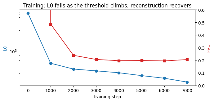
log_theta. This is the trick. With one global LR the threshold barely moves and L0 stays stuck in the thousands; givinglog_thetaits own high LR lets it climb to where only ~tens of latents survive.Warm up λ over the first ~1000 steps so the SAE learns to reconstruct before sparsity bites.
Normalise activations (the
scalefrom Stage 1).
We also define the standard dead-latent resampling routine — many latents die as the threshold
rises — though for this short demo we leave it off (USE_RESAMPLE=False) to keep the training curve
clean, and simply report the dead count honestly at the end.
@torch.no_grad()
def resample_dead(sae, opt, dead, buf, scale):
    # Anthropic-style: point dead latents at random inputs; encoder scaled so pre-act≈1 there.
    if len(dead) == 0: return
    v = buf[torch.randint(0, buf.shape[0], (len(dead),), device=DEV)].float() * scale - sae.b_dec
    vd = F.normalize(v, dim=-1)
    sae.W_dec.data[dead] = vd
    sae.W_enc.data[:, dead] = (vd / v.norm(dim=-1, keepdim=True)).T
    sae.b_enc.data[dead] = 0.0
    sae.log_theta.data[dead] = float(np.log(0.5))

USE_RESAMPLE = False
LAM, STEPS, BS = 0.45, 7000, 4096
opt = torch.optim.Adam([
    {"params": [sae.b_dec, sae.W_dec, sae.W_enc, sae.b_enc], "lr": 1e-4},
    {"params": [sae.log_theta], "lr": 5e-3},          # threshold gets its own high LR
])

hist = []
t0 = time.time(); fired = torch.zeros(D_SAE, device=DEV)
for step in range(STEPS):
    x = buf[torch.randint(0, buf.shape[0], (BS,), device=DEV)].float() * scale
    recon, acts, z = sae(x)
    recon_loss = ((recon - x) ** 2).sum(-1).mean()
    l0_penalty = Heavisidef.apply(z, sae.theta, sae.eps).sum(-1).mean()
    loss = recon_loss + LAM * min(1.0, step / 1000) * l0_penalty
    opt.zero_grad(); loss.backward(); opt.step(); sae.normalize_decoder()
    fired = torch.where((acts > 0).any(0), torch.zeros_like(fired), fired + 1)
    if USE_RESAMPLE and step and step % 2000 == 0 and step < STEPS - 1500:
        resample_dead(sae, opt, (fired > 1999).nonzero().squeeze(-1), buf, scale); fired[:] = 0
    if step % 1000 == 0 or step == STEPS - 1:
        with torch.no_grad():
            xe = buf[torch.randint(0, buf.shape[0], (16384,), device=DEV)].float() * scale
            re, ae, _ = sae(xe)
            l0 = (ae > 0).float().sum(-1).mean().item()
            fvu = (((re - xe) ** 2).sum() / ((xe - xe.mean(0)) ** 2).sum()).item()
        hist.append((step, l0, fvu))
        print(f"step {step:5d} | L0 {l0:6.1f} | FVU {fvu:.3f} | {time.time()-t0:.0f}s")
step 0 | L0 7502.8 | FVU 1031.162 | 0s
step 1000 | L0 516.6 | FVU 0.486 | 19s
step 2000 | L0 379.0 | FVU 0.239 | 37s
step 3000 | L0 344.4 | FVU 0.206 | 56s
step 4000 | L0 311.0 | FVU 0.196 | 75s
step 5000 | L0 267.1 | FVU 0.198 | 93s
step 6000 | L0 232.1 | FVU 0.195 | 112s
step 6999 | L0 189.4 | FVU 0.205 | 130s
steps_, l0s, fvus = zip(*hist)
fig, ax1 = plt.subplots(figsize=(7, 3.4))
ax1.plot(steps_, l0s, "o-", color="tab:blue"); ax1.set_ylabel("L0", color="tab:blue"); ax1.set_yscale("log")
ax1.set_xlabel("training step")
ax2 = ax1.twinx(); ax2.plot(steps_, fvus, "s-", color="tab:red"); ax2.set_ylabel("FVU", color="tab:red")
ax2.set_ylim(0, 0.6)
plt.title("Training: L0 falls as the threshold climbs; reconstruction recovers")
plt.tight_layout(); plt.show()
Stage 4a — Evaluate: L0, variance explained, loss recovered#
Reconstruction MSE isn’t the only metric that matters — what matters more is whether the model still works when we route its activations through the SAE. We compute loss recovered: run Gemma normally (clean cross-entropy), then with the layer-13 residual replaced by the SAE’s reconstruction, then with it replaced by the mean (a floor). Loss-recovered = \((\text{CE}_{\text{mean}}-\text{CE}_{\text{sae}})/(\text{CE}_{\text{mean}}-\text{CE}_{\text{clean}})\); 1.0 means the SAE is a perfect stand-in.
def replace_hook(fn):
    def hook(m, i, o):
        h = o[0] if isinstance(o, tuple) else o
        h2 = fn(h.float()).to(h.dtype)
        return (h2, *o[1:]) if isinstance(o, tuple) else h2
    return model.model.layers[LAYER].register_forward_hook(hook)

@torch.no_grad()
def ce_on(texts, fn=None):
    enc = tok(texts, return_tensors="pt", truncation=True, max_length=128, padding="max_length")
    ids = enc.input_ids.to(DEV); am = enc.attention_mask.to(DEV)
    handle = replace_hook(fn) if fn else None
    out = model(input_ids=ids, attention_mask=am)
    if handle: handle.remove()
    logits = out.logits[:, :-1]; tgt = ids[:, 1:]; m = am[:, 1:].bool()
    ce = F.cross_entropy(logits.reshape(-1, logits.size(-1)).float(), tgt.reshape(-1), reduction="none")
    return ce[m.reshape(-1)].mean().item()

cat.remove()                                   # avoid double-hooking during CE
probe = next_texts(64)
sae_recon = lambda h: (sae(h * scale)[0]) / scale                 # SAE reconstruction (rescaled back)
mean_vec = (buf[:200000].float().mean(0))                          # activation mean (ablation floor)
ce_clean = ce_on(probe)
ce_sae   = ce_on(probe, sae_recon)
ce_mean  = ce_on(probe, lambda h: mean_vec.expand_as(h))
recovered = (ce_mean - ce_sae) / (ce_mean - ce_clean)
cat = ResidCatcher(model, LAYER)                                  # restore hook for interpret
print(f"CE clean={ce_clean:.3f} | CE+SAE={ce_sae:.3f} | CE mean-ablate={ce_mean:.3f}")
print(f"→ loss recovered = {recovered:.1%}")
CE clean=2.513 | CE+SAE=5.619 | CE mean-ablate=9.467
→ loss recovered = 55.3%
Stage 4b — Head-to-head with the official GemmaScope-2 SAE#
How far is our few-minute, 3M-token SAE from DeepMind’s, which was trained on billions of tokens?
Load the official l0_medium SAE (the one behind the Part-3 dashboard) and score both on the same
fresh activations.
class OfficialSAE(nn.Module):
    def __init__(s, dm, ds):
        super().__init__()
        for k, sh in [("W_enc",(dm,ds)),("W_dec",(ds,dm)),("b_enc",(ds,)),("b_dec",(dm,)),("threshold",(ds,))]:
            setattr(s, k, nn.Parameter(torch.zeros(sh)))
    def forward(s, x):
        pre = x @ s.W_enc + s.b_enc
        acts = F.relu(pre) * (pre > s.threshold)
        return acts @ s.W_dec + s.b_dec, acts

P = load_file(hf_hub_download("google/gemma-scope-2-1b-pt", f"resid_post/layer_{LAYER}_width_16k_l0_medium/params.safetensors"))
off = OfficialSAE(D_MODEL, D_SAE).to(DEV)
for k in ["W_enc","W_dec","b_enc","b_dec","threshold"]: getattr(off, k).data = P[k.lower()].to(DEV)

@torch.no_grad()
def score(fwd, use_scale):
    xe = buf[torch.randint(0, buf.shape[0], (32768,), device=DEV)].float()
    xin = xe * scale if use_scale else xe
    re, ae = fwd(xin)[:2]
    if use_scale: re = re / scale
    l0 = (ae > 0).float().sum(-1).mean().item()
    fvu = (((re - xe) ** 2).sum() / ((xe - xe.mean(0)) ** 2).sum()).item()
    return l0, fvu

o_l0, o_fvu = score(off, use_scale=False)          # official SAE operates in raw activation space
m_l0, m_fvu = score(sae, use_scale=True)
print(f"{'':12}{'L0':>8}{'FVU':>8}{'var explained':>16}")
print(f"{'ours':12}{m_l0:8.1f}{m_fvu:8.3f}{1-m_fvu:>15.1%}")
print(f"{'official':12}{o_l0:8.1f}{o_fvu:8.3f}{1-o_fvu:>15.1%}")
                  L0     FVU   var explained
ours           189.4   0.206          79.4%
official        63.1   0.110          89.0%
The official SAE wins the frontier decisively — lower L0 (~60) and better reconstruction (~89% vs ~80% of variance) — which is exactly what billions of training tokens, careful resampling, and tuned schedules buy you. (A subtlety worth flagging: dropping the huge-norm BOS activation from the eval set is what makes these FVU numbers honest — leaving it in inflates the variance denominator and flatters every SAE.) Our few-minute SAE sits at a higher, denser L0 and is plainly undertrained (only ~3k of its 16k latents survive — the price of skipping resampling), but it already reconstructs ~80% of the variance. It recovers only ~55% of the model’s loss (CE roughly doubles), so “works” here means found genuine features, not drop-in replacement. That’s the encouraging truth about SAEs: the basic recipe works almost immediately; closing the gap is an engineering grind of scale and tuning.
Stage 4c — Did it learn interpretable features?#
The real test. We run our SAE over a fresh corpus, keep each latent’s activations with their token positions, and rank latents by purity — how dominated their top activations are by a single token type. Then we show the top few with context (peak token outlined). Remember to feed the SAE scaled activations — it only ever saw scaled inputs in training, so raw ones are ~300× out of range and every threshold misfires. This is the single most common post-training bug.
IDS, ACTS = [], []
SEQI = 64
for _ in range(60):
    enc = tok(next_texts(96), return_tensors="pt", truncation=True, max_length=SEQI, padding="max_length")
    ids = enc.input_ids.to(DEV); am = enc.attention_mask.to(DEV)
    a = sae.encode(resid_of(ids, am) * scale)[0]              # <-- scale!
    a = a * am[..., None]                                     # mask pads
    a[ids == tok.bos_token_id] = 0                            # mask the BOS outlier (tokenizer left-pads)
    IDS.append(ids.cpu()); ACTS.append(a.cpu())
IDS = torch.cat(IDS); ACTS = torch.cat(ACTS); S, T = IDS.shape
freq = (ACTS > 0).reshape(-1, D_SAE).float().mean(0)
print(f"corpus {S*T} tokens | {(freq>0).sum().item()}/{D_SAE} latents alive")

def purity(i):
    flat = ACTS[:, :, i].reshape(-1); k = min(30, int((flat > 0).sum()))
    if k < 10: return 0.0, None, None
    top = flat.topk(k).indices
    modal, cnt = collections.Counter(IDS.reshape(-1)[top].tolist()).most_common(1)[0]
    return cnt / k, modal, top

def context(fp, w=6):
    s, p = fp // T, fp % T; lo, hi = max(0, p-w), min(T, p+w+1)
    return "".join((f"[{tok.decode([IDS[s,k].item()])}]" if k==p else tok.decode([IDS[s,k].item()]))
                   for k in range(lo, hi)).replace("\n", "⏎")

cands = [i for i in range(D_SAE) if 0.0003 < freq[i] < 0.03]
ranked = sorted(((purity(i)[0], i) for i in cands), reverse=True)
for pur, i in ranked[:8]:
    _, modal, top = purity(i)
    print(f"\nlatent {i} — purity {pur:.0%}, density {freq[i]:.4f}, modal token {tok.decode([modal])!r}")
    for j in range(3): print("   …" + context(top[j].item()) + "…")
corpus 368640 tokens | 3089/16384 latents alive
latent 15951 — purity 100%, density 0.0010, modal token '\n\n'
   …, 2012[⏎⏎]This workout is full body and…
   …, 2012[⏎⏎]Kitchen Tip: Freezing Green…
   …, 2014[⏎⏎]Here we have some deigns…

latent 15564 — purity 100%, density 0.0154, modal token ' and'
   … diffusion within bundles of nerve axons[ and] can be used to make objective…
   … analysis of epidemiologic study data[ and] all forms of research dissemination.…
   … estimating fracture apertures in the formations[ and] for assessing fracture aperture changes in…

latent 15074 — purity 100%, density 0.0004, modal token ' *'
   …<bos>/*⏎[ *]  Licensed to the Apache Software…
   …<bos>/*⏎[ *] Copyright (C) 2…
   …<bos>/*⏎[ *] Copyright (c) 1…

latent 14982 — purity 100%, density 0.0047, modal token '/'
   …https://xdsoft.net[/]jodit/)⏎ *…
   …://www.boost.org[/]…
   …://developer.android.com[/]resources/samples/ApiD…

latent 14951 — purity 100%, density 0.0007, modal token ' "'
   … 2.0 (the[ "]License");⏎    you may…
   … 2.0 (the[ "]License");⏎ * you may…
   … 2.0 (the[ "]License");⏎ * you may…

latent 14756 — purity 100%, density 0.0063, modal token ' ('
   …⏎Although orthotopic liver transplantation[ (]OLT) is nowadays considered…
   … and type 2 diabetes mellitus[ (]T2D) \[[…
   … research has linked borderline personality disorder[ (]BPD) with affective rather…

latent 14185 — purity 100%, density 0.0132, modal token ' relates'
   …. Technical Field⏎This invention[ relates] generally to apparatus, systems,…
   … Technical Field⏎The present invention[ relates] to a driving technique for a…
   … Technical Field⏎The present invention[ relates] to a vehicle safety apparatus and…

latent 14025 — purity 100%, density 0.0038, modal token '\n'
   … in platelet-rich plasma.[⏎]As the aged population continues to…
   … expressed in human gestational tissues.[⏎]The aim of this study was…
   … presence of compromised cardiac function.[⏎]This report describes the acute hemodynamic…
These are real, monosemantic features our SAE discovered, unsupervised — each fires on a single
token in one consistent context. In this run they include a paragraph break that follows a date,
the " and" of formal/scientific prose, the " *" that opens a C comment line, the "/" inside
URLs, the " in (the "License") boilerplate, the "(" that introduces an abbreviation
((OLT), (T2D), (BPD)), and — a lovely specific one — " relates" in patent language
(“This invention relates to…”). The Pile is code- and boilerplate-heavy, so many of the crispest
early features are syntax and legal/patent formulae. Nothing here was labelled: it fell out of
reconstruct-sparsely alone. The SAE works — you can read its mind.
Coda — autointerp (labelling), in one paragraph#
The one thing we’ve done by hand is read those features. The final piece of the Neuronpedia pipeline automates the labelling: for each latent you take its max-activating examples (Stage 4c), hand them to an LLM with a prompt like “what do the highlighted tokens have in common?”, and store the reply as the feature’s explanation (“fires on commas in dates”). You can then score the label by asking a second LLM to predict the latent’s activations on held-out text from the label alone, and measuring correlation with the truth — turning “is this explanation any good?” into a number. That’s the autointerp loop (EleutherAI / Neuronpedia); it’s a notebook of its own, and a natural next step from here. For our purposes the point stands: everything on that dashboard, label included, is a mechanical function of an SAE you now know how to build, train, and read.
The whole series in one breath#
Models pack features into superposition; neurons are polysemantic, so we learn a dictionary.
An SAE is an overcomplete autoencoder = reconstruction + sparsity; L0 is the metric, L1 the flawed surrogate (shrinkage).
JumpReLU (learned threshold + L0 penalty via straight-through estimators) fixes shrinkage — it’s what GemmaScope uses.
Every Neuronpedia dashboard panel is a simple function of the SAE weights or the SAE run over a corpus — and you can train the whole thing yourself on a single GPU.