

SAE architectures & JumpReLU — the activation GemmaScope uses#
Part 2 of 4. In Part 1 we built a plain ReLU SAE with an L1 sparsity penalty and watched it recover features from superposition. We also flagged a tension: we want to control L0 (the count of active latents) but we can only train against L1 (the sum of magnitudes). That mismatch has a concrete, damaging side-effect — shrinkage — and fixing it is what the modern SAE zoo (TopK, Gated, JumpReLU) is all about.
This notebook:
demonstrates the L1 shrinkage / feature-suppression problem quantitatively,
surveys the fixes (TopK, Gated, JumpReLU),
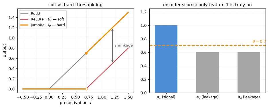
shows why a threshold is the right tool — encoder scores are true signal plus positive leakage from non-orthogonal features; hard vs soft thresholding,
implements JumpReLU properly — including its straight-through-estimator gradients, by hand — and shows it removes shrinkage,
and connects to GemmaScope, whose exact forward pass we’ll load in Part 3.
Runs on CPU in well under a minute.
1. The problem with L1: shrinkage#
Look again at the ReLU SAE loss:
The L1 term penalises every unit of activation, including the activations we want to keep. So for a latent that genuinely should fire, the optimiser faces a tug of war: turning it up improves reconstruction but costs \(\lambda\) per unit. The compromise is to make the activation smaller than it should be. This is activation shrinkage (a.k.a. feature suppression): the SAE systematically under-estimates how strongly each feature is present. The direction (which feature) is right; the magnitude is biased low.
We can measure it exactly on the Part-1 toy, because there we know the true magnitude of each active feature. Plot the SAE’s recovered activation against the true magnitude, for a well-matched latent, and read off the slope: slope 1 = unbiased, slope < 1 = shrinkage.
import numpy as np, torch, torch.nn as nn, torch.nn.functional as F
import matplotlib.pyplot as plt
torch.manual_seed(0)

# --- same known-dictionary generator as Part 1 ---
d, n_true, d_sae = 16, 32, 64
D_true = F.normalize(torch.randn(n_true, d), dim=-1)
p_active = 3.0 / n_true
def gen(b):
    m = (torch.rand(b, n_true) < p_active).float()
    mags = (0.5 + torch.rand(b, n_true)) * m
    return mags @ D_true, mags

class ReLUSAE(nn.Module):
    def __init__(self):
        super().__init__()
        self.b_dec = nn.Parameter(torch.zeros(d))
        self.W_enc = nn.Parameter(torch.randn(d, d_sae) / np.sqrt(d))
        self.b_enc = nn.Parameter(torch.zeros(d_sae))
        self.W_dec = nn.Parameter(F.normalize(torch.randn(d_sae, d), dim=-1))
    @torch.no_grad()
    def nd(self): self.W_dec.data = F.normalize(self.W_dec.data, dim=-1)
    def forward(self, x):
        f = F.relu((x - self.b_dec) @ self.W_enc + self.b_enc)
        return f @ self.W_dec + self.b_dec, f

def train_relu(sae, l1, steps=2500, lr=4e-3):
    opt = torch.optim.Adam(sae.parameters(), lr=lr)
    for _ in range(steps):
        x, _ = gen(4096); xh, f = sae(x)
        (((xh - x) ** 2).sum(-1).mean() + l1 * f.abs().sum(-1).mean()).backward()
        opt.step(); opt.zero_grad(); sae.nd()
    return sae

def shrinkage_pairs(sae):
    # (true magnitude, sae activation) over all matched, active feature/latent pairs
    x, mags = gen(16384)
    with torch.no_grad(): a = sae(x)[1]          # (recon, f) -> f
    cos = F.normalize(D_true, dim=-1) @ F.normalize(sae.W_dec, dim=-1).T
    bv, bi = cos.max(1); tm, sm = [], []
    for j in range(n_true):
        if bv[j] < 0.9: continue
        on = mags[:, j] > 0
        tm.append(mags[on, j]); sm.append(a[on, bi[j].item()])
    tm, sm = torch.cat(tm), torch.cat(sm)
    A = torch.stack([tm, torch.ones_like(tm)], 1)
    slope, intcpt = torch.linalg.lstsq(A, sm).solution.tolist()
    l0 = (a > 0).float().sum(-1).mean().item()
    return tm, sm, slope, intcpt, l0

relu_sae = train_relu(ReLUSAE(), l1=0.8)
tm_r, sm_r, slope_r, int_r, l0_r = shrinkage_pairs(relu_sae)
print(f"ReLU SAE:  L0={l0_r:.1f}   recovered ≈ {slope_r:.2f} × true magnitude  (slope<1 ⇒ shrinkage)")
ReLU SAE: L0=5.3 recovered ≈ 0.64 × true magnitude (slope<1 ⇒ shrinkage)
The ReLU SAE recovers only ~65% of each feature’s true magnitude — a large, systematic bias. In a real model this means downstream analyses that use SAE activation values (steering strengths, attributions) are all mis-scaled.
Why not just… not penalise magnitude?#
Because the penalty is doing two jobs at once: (a) deciding which latents are on (the part we want) and (b) squashing how big the on-latents are (the part we don’t). We want to keep (a) and drop (b). Every architecture below is a different way to separate those two jobs.
2. The fixes, at a glance#
Architecture |
Activation / mechanism |
Sparsity control |
Idea |
|---|---|---|---|
ReLU + L1 (baseline) |
\(\operatorname{ReLU}(W_{\text{enc}}x+b)\) |
L1 penalty \(\lambda\lVert f\rVert_1\) |
simple, but L1 causes shrinkage; L0 only controlled indirectly via \(\lambda\) |
TopK |
keep the \(k\) largest pre-activations, zero the rest |
exact: L0 \(=k\) by construction |
no magnitude penalty ⇒ no shrinkage; but \(k\) is fixed per token (can’t spend fewer/more) |
Gated |
separate gate (which latents fire) from magnitude (how much) — two encoder paths |
L1 on the gate path only |
decouples the two jobs explicitly; needs an auxiliary loss; trains well |
JumpReLU |
\(\operatorname{JumpReLU}_\theta(z)=z\cdot\mathbb{1}[z>\theta]\), learned per-latent threshold \(\theta\) |
L0 penalty directly \(\lambda\lVert f\rVert_0\) |
a ReLU with a learned “on” threshold; penalise the count, not the magnitude |
TopK’s catch (beyond the table): every token uses exactly \(k\) latents — one that needs only 2 features still burns \(k\), and one that needs \(2k\) can’t have them.
Gated and JumpReLU both let L0 vary per token while avoiding shrinkage. They’re closely related: with a bit of weight-tying a Gated SAE is a JumpReLU SAE. GemmaScope chose JumpReLU, so that’s what we build.
3. Why a threshold? Leakage is often positive#
In Part 1 the ReLU cleaned up interference — but only because those toys embedded features antipodally, so the interference landed on the negative side. Real overcomplete dictionaries aren’t that kind. Think of the encoder as a bank of matched filters: latent \(i\) scores the activation by dot product with its feature direction,
true signal plus leakage from every correlated feature. An overcomplete dictionary cannot be orthogonal, so some \(d_i^\top d_j \neq 0\) — and their signs are whatever geometry dictates.
Concretely: three unit-norm features in 2-D, with only feature 1 active,
The \(0.6\)s are pure leakage — and positive, so ReLU keeps them: it is the maximally permissive detector, “activate on any positive correlation”. What separates signal from leakage here is not sign but size. A threshold \(\theta = 0.7\) recovers \(z = (1,0,0)\) exactly, and works whenever sparsity keeps the accumulated leakage below the true activations:
But how you threshold matters:
score \(a\) |
ReLU |
\(\operatorname{ReLU}(a-0.7)\) — soft |
\(\operatorname{JumpReLU}_{0.7}\) — hard |
|---|---|---|---|
\(0.6\) (leakage) |
\(0.6\) |
\(0\) |
\(0\) |
\(1.2\) (signal) |
\(1.2\) |
\(\mathbf{0.5}\) |
\(\mathbf{1.2}\) |
Folding the threshold into the encoder bias, \(\operatorname{ReLU}(a-\theta)\), is soft thresholding: it rejects the leakage, but it also subtracts \(\theta\) from every genuine activation — that is exactly §1’s shrinkage, rebuilt by hand. JumpReLU is hard thresholding: below \(\theta\), off; above \(\theta\), full magnitude. This is textbook sparse denoising — discard small coefficients as leakage, keep large ones untouched — except the basis is learned and overcomplete, with one learned threshold per latent.
import numpy as np, matplotlib.pyplot as plt

# 3 unit-norm feature directions in 2-D — overcomplete, so they can't be orthogonal
D = np.array([[1.0, 0.6,  0.6],
              [0.0, 0.8, -0.8]])
x = D @ np.array([1.0, 0.0, 0.0])   # only feature 1 is active
a = D.T @ x                          # matched-filter scores  a_i = d_i . x
theta = 0.7
print("scores     a =", a, "  <- the 0.6s are pure (positive!) leakage")
print("ReLU         :", np.maximum(a, 0))
print("soft, a-theta:", np.maximum(a - theta, 0))
print("hard/JumpReLU:", a * (a > theta))

fig, axes = plt.subplots(1, 2, figsize=(9.5, 3.9))

# left: the three gates as transfer curves
u = np.linspace(-0.5, 1.5, 401)
ax = axes[0]
ax.plot(u, np.maximum(u, 0), color="0.55", lw=2, label="ReLU")
ax.plot(u, np.maximum(u - theta, 0), color="#d1495b", lw=2, label=r"ReLU$(a-\theta)$ — soft")
ax.plot([-0.5, theta], [0, 0], color="#f08c00", lw=2.6)
ax.plot([theta, 1.5], [theta, 1.5], color="#f08c00", lw=2.6, label=r"JumpReLU$_\theta$ — hard")
ax.scatter([theta], [theta], s=30, color="#f08c00", zorder=3)
ax.scatter([theta], [0], s=30, facecolor="white", edgecolor="#f08c00", zorder=3)
ax.axvline(theta, color="0.8", lw=0.8, ls=":")
ax.annotate("", xy=(1.2, 1.2), xytext=(1.2, 0.5),
            arrowprops=dict(arrowstyle="<->", color="0.35", lw=1.2))
ax.text(1.24, 0.83, "shrinkage", fontsize=9, color="0.35")
ax.set_xlabel("pre-activation $a$"); ax.set_ylabel("output")
ax.set_title("soft vs hard thresholding", fontsize=11)
ax.legend(fontsize=9, loc="upper left"); ax.grid(alpha=0.25, ls=":")

# right: the worked example — what the threshold must separate
ax = axes[1]
ax.bar(range(3), a, width=0.55, color=["#4c8dd6", "0.65", "0.65"])
ax.axhline(theta, color="#f08c00", lw=2, ls="--")
ax.text(2.42, theta + 0.04, r"$\theta = 0.7$", color="#f08c00", ha="right", fontsize=10)
ax.set_xticks(range(3), ["$a_1$ (signal)", "$a_2$ (leakage)", "$a_3$ (leakage)"], fontsize=9)
ax.set_ylim(0, 1.25)
ax.set_title("encoder scores: only feature 1 is truly on", fontsize=11)
ax.grid(alpha=0.25, ls=":", axis="y")

fig.tight_layout(); plt.show()
scores     a = [1.  0.6 0.6]   <- the 0.6s are pure (positive!) leakage
ReLU         : [1.  0.6 0.6]
soft, a-theta: [0.3 0.  0. ]
hard/JumpReLU: [1. 0. 0.]
4. JumpReLU in depth#
The JumpReLU activation is a ReLU with a learned threshold \(\theta_i\) per latent:
Below the threshold the latent is exactly off; above it, the latent passes through at full magnitude (no shrinkage). Sparsity is now controlled by penalising the L0 count directly:
This is exactly the thing we said we wanted in Part 1. So what was stopping us? The gradients are dead. Both \(H(z-\theta)\) (a step) and \(\lVert f\rVert_0\) (a count) are piecewise-constant in \(\theta\), so \(\partial/\partial\theta = 0\) almost everywhere — the threshold would never move.
Straight-through estimators (STE)#
The trick: in the backward pass, replace the useless zero-derivative with a pseudo-derivative that’s a narrow bump around the discontinuity. Concretely, DeepMind use a rectangle kernel \(K(u)=\mathbb{1}[|u|<\tfrac12]\) of bandwidth \(\varepsilon\), and define:
Intuition: nudging \(\theta\) only matters for inputs \(z\) sitting right at the threshold (within \(\varepsilon\)). For those, lowering \(\theta\) turns the latent on (gaining a count of 1, or a magnitude of \(\theta\)); the kernel concentrates that effect in a narrow window of width \(\varepsilon\) around \(\theta\). For the input \(z\) we keep the honest derivatives (\(\partial H/\partial z:=0\), \(\partial\operatorname{JumpReLU}/\partial z:=\mathbb{1}[z>\theta]\)) so that \(\theta\) is the only parameter that implements thresholding.
We implement both as custom torch.autograd.Functions with different forward/backward behaviour.
def rectangle(x, width=1.0):
    return (x.abs() < width / 2).float()

class Heaviside(torch.autograd.Function):
    # forward: 1[z > θ];   backward: dH/dz := 0,  dH/dθ := -(1/ε)·K((z-θ)/ε)
    @staticmethod
    def forward(ctx, z, theta, eps):
        ctx.save_for_backward(z, theta); ctx.eps = eps
        return (z > theta).float()
    @staticmethod
    def backward(ctx, grad_out):
        z, theta = ctx.saved_tensors; eps = ctx.eps
        grad_theta = -(1.0 / eps) * rectangle((z - theta) / eps) * grad_out
        return 0.0 * grad_out, grad_theta, None

class JumpReLU(torch.autograd.Function):
    # forward: z·1[z > θ];   backward: dJ/dz := 1[z>θ],  dJ/dθ := -(θ/ε)·K((z-θ)/ε)
    @staticmethod
    def forward(ctx, z, theta, eps):
        ctx.save_for_backward(z, theta); ctx.eps = eps
        return z * (z > theta).float()
    @staticmethod
    def backward(ctx, grad_out):
        z, theta = ctx.saved_tensors; eps = ctx.eps
        grad_z = (z > theta).float() * grad_out
        grad_theta = -(theta / eps) * rectangle((z - theta) / eps) * grad_out
        return grad_z, grad_theta, None

# --- unit tests (from the DeepMind/ARENA conventions) ---
z = torch.tensor([[1.0, 1.4, 1.6, 2.0]], requires_grad=True)
theta = torch.tensor([1.5, 1.5, 1.5, 1.5], requires_grad=True)
out = JumpReLU.apply(z, theta, 0.5); out.backward(torch.ones_like(out))
torch.testing.assert_close(out, torch.tensor([[0.0, 0.0, 1.6, 2.0]]))            # z·1[z>θ]
torch.testing.assert_close(theta.grad, torch.tensor([0.0, -3.0, -3.0, 0.0]))     # -θ/ε·K
torch.testing.assert_close(z.grad, torch.tensor([[0.0, 0.0, 1.0, 1.0]]))         # 1[z>θ]
print("JumpReLU forward & straight-through gradients: tests passed ✓")
JumpReLU forward & straight-through gradients: tests passed ✓
A JumpReLU SAE#
Now assemble the SAE. Two implementation details that matter (both from the GemmaScope / DeepMind appendix):
Parameterise the threshold as \(\theta=\exp(\log\theta)\) so it stays positive and the learnable parameter is unconstrained.
Feed \(\operatorname{ReLU}(\text{pre})\) (not the raw pre-activation) into the JumpReLU/Heaviside, so negative pre-activations can’t leak gradient into \(\theta\) in edge cases.
class JumpReLUSAE(nn.Module):
    def __init__(self, eps=0.02, theta0=0.05):
        super().__init__(); self.eps = eps
        self.b_dec = nn.Parameter(torch.zeros(d))
        self.W_enc = nn.Parameter(torch.randn(d, d_sae) / np.sqrt(d))
        self.b_enc = nn.Parameter(torch.zeros(d_sae))
        self.W_dec = nn.Parameter(F.normalize(torch.randn(d_sae, d), dim=-1))
        self.log_theta = nn.Parameter(torch.full((d_sae,), float(np.log(theta0))))
    @property
    def theta(self): return self.log_theta.exp()
    @torch.no_grad()
    def nd(self): self.W_dec.data = F.normalize(self.W_dec.data, dim=-1)
    def forward(self, x):
        pre = (x - self.b_dec) @ self.W_enc + self.b_enc           # pre-activations
        z = F.relu(pre)                                            # z = ReLU(pre-acts) — the value we threshold
        acts = JumpReLU.apply(z, self.theta, self.eps)             # pass z only where z > θ (at full magnitude)
        return acts @ self.W_dec + self.b_dec, acts, z

def train_jump(sae, lam, steps=2500, lr=4e-3):
    opt = torch.optim.Adam(sae.parameters(), lr=lr)
    for _ in range(steps):
        x, _ = gen(4096); xh, acts, z = sae(x)
        l0_pen = Heaviside.apply(z, sae.theta, sae.eps).sum(-1).mean()   # count of active latents — Heaviside (not z>0) so the STE gradient can still reach θ
        (((xh - x) ** 2).sum(-1).mean() + lam * l0_pen).backward()
        opt.step(); opt.zero_grad(); sae.nd()
    return sae

jump_sae = train_jump(JumpReLUSAE(), lam=0.15)

# reuse the shrinkage probe (works for any SAE returning (recon, acts, ...))
def shrink_pairs(sae):
    x, mags = gen(16384)
    with torch.no_grad(): acts = sae(x)[1]
    cos = F.normalize(D_true, dim=-1) @ F.normalize(sae.W_dec, dim=-1).T
    bv, bi = cos.max(1); tm, sm = [], []
    for j in range(n_true):
        if bv[j] < 0.9: continue
        on = mags[:, j] > 0
        tm.append(mags[on, j]); sm.append(acts[on, bi[j].item()])
    tm, sm = torch.cat(tm), torch.cat(sm)
    A = torch.stack([tm, torch.ones_like(tm)], 1)
    slope, intcpt = torch.linalg.lstsq(A, sm).solution.tolist()
    l0 = (acts > 0).float().sum(-1).mean().item()
    return tm, sm, slope, l0

tm_j, sm_j, slope_j, l0_j = shrink_pairs(jump_sae)
print(f"JumpReLU SAE:  L0={l0_j:.1f}   recovered ≈ {slope_j:.2f} × true magnitude  (slope≈1 ⇒ no shrinkage)")
JumpReLU SAE: L0=2.9 recovered ≈ 0.91 × true magnitude (slope≈1 ⇒ no shrinkage)
# side-by-side: recovered activation vs true magnitude
fig, ax = plt.subplots(1, 2, figsize=(11, 4.2), sharex=True, sharey=True)
for a_, tm, sm, slope, l0, name in [
    (ax[0], tm_r, sm_r, slope_r, l0_r, "ReLU + L1"),
    (ax[1], tm_j, sm_j, slope_j, l0_j, "JumpReLU + L0"),
]:
    a_.scatter(tm, sm, s=3, alpha=0.15, color="darkorange")
    xs = torch.linspace(0, 1.6, 20)
    a_.plot(xs, xs, "k--", lw=1, label="unbiased (slope 1)")
    a_.plot(xs, slope * xs, "b-", lw=1.5, label=f"fit (slope {slope:.2f})")
    a_.set_title(f"{name}   (L0≈{l0:.1f})"); a_.set_xlabel("true feature magnitude")
    a_.legend(loc="upper left", fontsize=8)
ax[0].set_ylabel("SAE recovered activation")
plt.tight_layout(); plt.show()
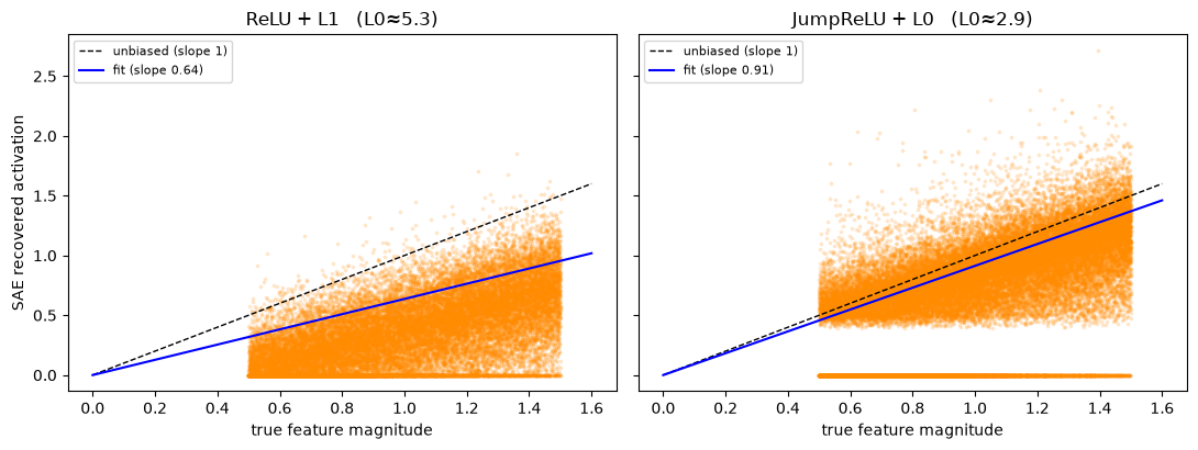
Same reconstruction task — and JumpReLU is if anything sparser (L0 2.9 vs 5.3) — yet the ReLU cloud sits well below the diagonal (slope ≈ 0.65) while the JumpReLU cloud hugs it (slope ≈ 0.9–1.0). JumpReLU removed the shrinkage bias because it never penalises magnitude, only the count of active latents. (The slight negative intercept is the threshold zeroing weak activations — pinning the low end at zero, not shrinking the survivors.)
5. The frontier: same reconstruction at lower L0#
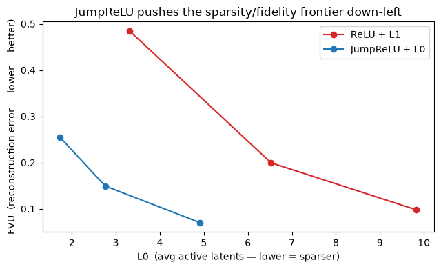
The other benefit is a better L0-vs-reconstruction trade-off. Sweep the sparsity coefficient for each architecture and plot the frontier — down-and-left is better (fewer active latents for the same error).
def eval_sae(sae):
    x, _ = gen(16384)
    with torch.no_grad(): xh, acts, *_ = sae(x)
    l0 = (acts > 0).float().sum(-1).mean().item()
    fvu = (((xh - x) ** 2).sum() / ((x - x.mean(0)) ** 2).sum()).item()
    return l0, fvu

relu_pts = [eval_sae(train_relu(ReLUSAE(), l1, steps=1500)) for l1 in [0.3, 0.6, 1.2]]
jump_pts = [eval_sae(train_jump(JumpReLUSAE(), lam, steps=1500)) for lam in [0.08, 0.2, 0.5]]

plt.figure(figsize=(6.5, 4))
for pts, name, c in [(relu_pts, "ReLU + L1", "tab:red"), (jump_pts, "JumpReLU + L0", "tab:blue")]:
    pts = sorted(pts); xs = [p[0] for p in pts]; ys = [p[1] for p in pts]
    plt.plot(xs, ys, "o-", color=c, label=name)
plt.xlabel("L0  (avg active latents — lower = sparser)")
plt.ylabel("FVU  (reconstruction error — lower = better)")
plt.title("JumpReLU pushes the sparsity/fidelity frontier down-left")
plt.legend(); plt.tight_layout(); plt.show()
6. GemmaScope: JumpReLU at scale#
GemmaScope
is DeepMind’s open release of hundreds of JumpReLU SAEs for the Gemma models — every layer,
several widths, and the GemmaScope-2 update covers Gemma 3 (including the
gemma-3-1b-pt model we’ll use). Everything in this notebook is exactly what’s under the hood,
with three scaling-up details:
Width & L0. Our target SAE is
resid_post, layer 13, width 16384 (16k), trained to L0 ≈ 60. Each (layer, width) is released at several L0 points (l0_small / medium / big); Neuronpedia serves the medium one for our dashboard.The exact forward pass. GemmaScope’s stored parameters are
w_enc, w_dec, b_enc, b_dec, threshold, and the forward is precisely:pre = x @ W_enc + b_enc acts = relu(pre) * (pre > threshold) # JumpReLU with a *fixed* learned threshold recon = acts @ W_dec + b_dec
At inference the STE machinery is gone —
thresholdis just a constant vector. The STE only existed to train those thresholds. (We’ll load these real weights in Part 3.)Targeting a specific L0. Rather than hunting \(\lambda\), you can penalise the squared distance to a target, \(\lambda\big(\lVert f\rVert_0 / L_0^{\text{target}} - 1\big)^2\), which lets you dial in “L0 ≈ 60” directly. GemmaScope-style training also normalises activations (so \(\mathbb{E}\lVert x\rVert=\sqrt{d_{\text{model}}}\)), warms up the sparsity coefficient, and resamples dead latents — all of which we’ll do for real in Part 4.
A caveat worth internalising: JumpReLU SAEs are harder to train than the maths suggests — several groups struggled to reproduce DeepMind’s results, largely because of the threshold gradient. Our from-scratch run in Part 4 will hit the same issues (dead latents, L0 that overshoots) and show the fixes.
Recap & what’s next#
L1 causes shrinkage: the penalty on magnitude biases recovered activations low (slope ≈ 0.65 on our toy).
Why a threshold: overcomplete dictionaries leak — an encoder score is true signal plus interference from correlated features, and the leakage is often positive, so ReLU keeps it. Soft thresholding (fold \(\theta\) into the bias) rejects leakage but shrinks; hard thresholding (JumpReLU) rejects leakage at full magnitude.
TopK / Gated / JumpReLU separate “which latents fire” from “how big they are”. JumpReLU = ReLU with a learned per-latent threshold + a direct L0 penalty, trained via straight-through estimators with a rectangle kernel.
JumpReLU removes shrinkage (slope ≈ 1) and improves the L0/fidelity frontier — which is why GemmaScope uses it.
Next → Part 3: Reconstructing the Neuronpedia dashboard. We load the real GemmaScope-2 SAE for Gemma 3, run Gemma 3 1B on text, and rebuild every panel of the latent-7447 dashboard — top logits, activation density, max-activating examples, cosine neighbours — from scratch.